In this post we will talk about the Bias-Variance tradeoff, explaining where it comes from and how we can manage it, introducing techniques for model selection (feature selection, regularization, dimensionality reduction) and model ensemble (bagging and boosting).
Disclaimer: the following notes were written following the slides provided by the professor Restelli at Polytechnic of Milan and the book ‘Pattern Recognition and Machine Learning'.
Bias-Variance trade-off and Model Selection
No Free Lunch Theorems
Define $Acc_G(L)$ as the generalization accuracy of the learner $L$, which is the accuracy of $L$ on non-training samples. $\mathcal{F}$ is the set of all possible concepts, $y = f(x)$, that are the true models we want to learn.
Theorem For any learner $L$, $\frac{1}{|\mathcal{F}|}\sum_{\mathcal{F}}Acc_G(L) = \frac{1}{2}$ (given any distribution $\mathcal{P}$ over $\boldsymbol{x}$ and the training set size $N$)
This means that any learner, on average of all the models, has the same accuracy of random sampling, and so what is learned from the seen data is useless for predicting new data. If this is true, well…why does Machine Learning exist?
The point here is that highlighted “on average”. Indeed, Machine Learning is based on the assumption that not all the models are equally likely, because the seen data are related to the unseen data, so the distribution over models is restricted after seeing the data. In practice, Machine Learning is betting that some models are better than others (in that specific case), in the same way you assume that there is some regularity in the world, so that what you observe is meaningful for what you want to predict.
Corollary For any two learners $L_1, L_2$: if $\exists$ learning problems s.t. $Acc_G(L_1) > Acc_G(L_2)$, then $\exists$ learning problems s.t. $Acc_G(L_2) > Acc_G(L_1)$
This means that there is no best method for solving all the machine learning problems, because every method is based on some assumptions and it can perform better only on some subset of models. This is the reason for which there isn’t an unique algorithm for solving all the ML problems.
Bias-Variance trade-off
As we have seen in past chapters, the use of maximum likelihood, or equivalently least squares, can lead to overfitting if complex models are trained using datasets of limited size. On the other hand, limiting the number of basis functions in order to avoid this problem has the side effect of making our model less flexible and so less capable of capturing interesting trends in data. We also introduced regularization to control overfitting for models with many parameters, but this solution raises the question of how to determine a suitable value for the regularization coefficient $\lambda$.
For all these reasons, we showed a valid alternative, represented by the Bayesian setting. However, let’s now investigate a frequentist viewpoint of the complexity model issue, knows as the bias-variance trade-off.
Assume that we have a dataset $D$ with $N$ samples obtained by a function $t_i = f(\boldsymbol{x_i}) + \epsilon$ with $E[\epsilon] = 0$ and $Var[\epsilon] = \sigma^2$. We want to find a model $y(\boldsymbol{x})$ that approximates $f$ as well as possible. Consider the expected square error on an unseen sample $x$:
$$ \displaylines{E[(t - y(x))^2] = E[t^2 + y(x)^2 -2ty(x)] \\ = E[t^2] + E[y(x)^2] - E[2ty(x)] \\ = E[t^2] \pm E[t]^2 + E[y(x)^2] \pm E[y(x)]^2 - 2f(x)E[y(x)] \\ = Var[t] + E[t]^2 + Var[y(x)] + E[y(x)]^2 - 2f(x)E[y(x)] \\ = Var[t] + Var[y(x)] + E[f(x)-y(x)]^2} $$
where:
- $Var[t] = \sigma^2$ is the irreducible noise.
- $Var[y(x)]$ is the $Variance$, that measures how much the solutions for individual data sets vary around their average.
- $E[f(x)-y(x)]^2$ is the $Bias^2$, that represents the difference between the average prediction over all data sets and the true function.
Substantially, $expected \ loss = noise + variance + (bias)^2$
A high bias means that even with a lot of samples it is not possible to learn the true model (underfitting). It decreases with more complex models.
A high variance means that the model depends highly on noise and so its solutions vary a lot depending on the particular choice of the data sets (overfitting). It can decrease by using simpler models or with more samples.
Increasing the number of samples is the only way in which we can reduce the variance while keeping the bias unchanged, but of course this is not always possible.
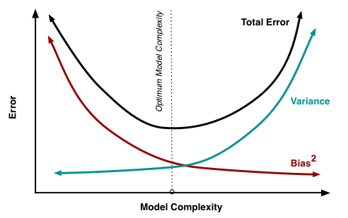
Our goal is to minimize the expected loss and, as we can see from the image above, there is a clear trade-off between variance and bias, leading to very flexible models having low bias and high variance, and relatively rigid models having high bias and low variance.
The bias-variance tradeoff can be managed using different techniques:
- Model selection
- Feature selection
- Regularization
- Dimension reduction
- Model ensemble
- Bagging
- Boosting
Model Selection
The variance-bias trade-off becomes even more problematic when we have to deal with high-dimensional data, since the risk of overfitting is higher, the number of required samples is larger and the computational cost increases.
So, if we can’t solve a problem with few features, adding more features could not be a good idea, especially if the number of samples stays the same.
Feature Selection
It identifies a subset of features which are the most related to the output. Feature selection techniques are used for four reasons:
- simplification of models to make them easier to interpret by researchers/users
- shorter training times
- to avoid the curse of dimensionality
- enhanced generalization by reducing overfitting (formally, reduction of variance)
The best subset selection method is to try all the possible combinations of features. Of course, this approach has problems of high computational cost and overfitting if the number of features is large. There exists some metaheuristics to mitigate these issues:
- Filter: rank the features and select the best ones;
- Embedded: the learning algorithm exploits its own variable selection technique (Lasso, Decision Trees, Auto-encoding, etc.);
- Wrapper: evaluate only some subsets:
- Forward step-wise selection: starts from an empty model and adds features one at a time;
- Backward step-wise selection: starts with all the features and removes the least useful one at a time.
How can we see how well our model performs on the test set?
Direct estimation Randomly split the data set into training set, validation set and test set and use the validation set to tune the learning algorithm. In this case cross-validation is used to prevent overfitting over the validation set (if it is not big enough).
-
Leave-One-Out Cross Validation (LOO) uses a validation set $\{n\}$ with 1 example extracted from the dataset $D$ and learns the model with $D \setminus \{n\}$ dataset. The process is repeated for all the $N$ points of the dataset and the error is averaged
$$L_{LOO} = \frac{1}{N}\sum_{n=1}^{N}(t_n-y_{\mathcal{D}\setminus{n}}(\boldsymbol{x_n}))^2$$
-
k-fold Cross Validation randomly divides the training data into $k$ equal parts: $D_1,…,D_k$ and for each $i$:
-
learns the model $y_{\mathcal{D}\setminus{D_i}}$
-
estimates the error of $y_{\mathcal{D}\setminus{D_i}}$ on validation set $D_i$
$$L_{D_i} = \frac{k}{N}\sum_{(\boldsymbol{x_n},t_n)\in\mathcal{D_i}}(t_n-y_{\mathcal{D}\setminus{D_i}}(\boldsymbol{x_n}))^2$$
-
all the $k$ errors are averaged
$L_{k-fold} = \frac{1}{k}\sum_{i=1}^{k}L_{\mathcal{D_i}}$
Usually $k = 10$ is used.
-
k-fold Cross Validation is much faster than LOO, but it is more (pessimistically) biased.
In addition to these two methods, there are other techniques, called Adjustment Techniques, that are usually used when we have a small dataset and a complex model. Some of them are: $AIC, BIC, Adjusted \ R^2$…
Regularization
We already spoke about Ridge regression and Lasso in the “Linear Regression” chapter. These methods can significanlty reduce the variance, but unfortunately, at the same time, they increase bias, because the penalization in the loss function modifies the objective of the optimization and so, even with infinite samples, it would be impossible to obtain a perfect solution. This is the reason why regularization should not be used when a lot of samples are available.
Dimension reduction
Dimension reduction (or dimensionality reduction) methods, differently from the previous approaches, transform the original features and then the model is learned on the transformed variable.
The basic idea is less features but with the same amount of information (more or less).
Principal Component Analysis (PCA) Principal component analysis (PCA) simplifies the complexity in high-dimensional data while retaining trends and patterns. It does this by transforming the data into fewer dimensions, which act as summaries of features.
It can be divided in the following steps:
- Compute the mean of the data $\boldsymbol{\bar{x}} = \frac{1}{N}\sum_{n=1}^{N}\boldsymbol{x_n}$
- Subtract the mean: for PCA to work properly, you have to subtract the mean from each of the data dimensions. This produces a data set whose mean is zero
- Calculate the covariance matrix $\boldsymbol{S} = \boldsymbol{X}^T\boldsymbol{X} = \frac{1}{N-1}\sum_{n=1}^{N}(\boldsymbol{x_n}-\boldsymbol{\bar{x}})(\boldsymbol{x_n}-\boldsymbol{\bar{x}})^T$
- Calculate the eigenvectors and eigenvalues of the covariance matrix
It turns out that the eigenvector with the highest eigenvalue is the principle component of the data set. In general, once eigenvectors are found from the covariance matrix, the next step is to order them by eigenvalue, highest to lowest. This gives you the components in order of significance. Now, if you like, you can decide to ignore the components of lesser significance.
- Form a feature vector: constructed by taking the eigenvectors that you want to keep from the list of eigenvectors, and forming a matrix with these eigenvectors in the columns.
- Derive the new dataset: $new \ dataset = feature \ vector^T \times zero \ mean \ data$
PCA can be analyzed much more in details, so this is a link to go deeper: PCA
PCA has multiple benefits:
- helps to reduce the computational complexity
- can help supervised learning, because reduced dimensions allow simpler hypothesis spaces and less risk of overfitting
- can be used for noise reduction
But also some drawbacks:
- fails when data consists of multiple clusters
- the directions of greatest variance may not be the most informative
- computational problems with many dimensions
- PCA computes linear combination of features, but data often lie on a nonlinear manifold. Suppose for example that the data are distributed on two dimensions as a circumference: it can be actually represented by one dimension, but PCA is not able to capture it.
Model Ensembles
We now introduce meta-algorithms, which instead of learning one model, learn several and combine them.
Bagging
This algorithm reduces the variance without increasing the bias, but the variance needs to be high initially in order to see considerable improvements. It is based on the principle that averaging over multiple models reduces the variance:
$Var(\bar{X}) = \frac{Var(X)}{N}$
Actually this is not the real reduction because it is based on the assumption that the models are independent.
To be able to train multiple models from a unique train set, bootstrapping is performed: generate B bootstrap samples of the training data by random sampling with replacement. Then train a model for each bootstrap sample and the prediction will be determined through majority vote in case of classification or through average of the predicted values in case of regression. It improves the performance for unstable learners which vary significantly with small changes in the data set.
Note that Bagging is relatively easy to parallelize because all the models work on the same problem independently.
Random Forest is an extension over bagging. It takes one extra step where in addition to taking the random subset of data, it also takes the random selection of features rather than using all features to grow trees.
Boosting
The aim of boosting is to reduce the bias without increasing the variance (too much). It works by sequentially training weak learners, i.e. learners that have a performance that on any train set is slightly better than chance prediction (high bias).
The steps are the following:
- Weight all the train samples equally
- Train a weak model on the train set (since it is weak, it will perform good on some samples and bad on another)
- Compute the error of the model on the train set
- Increase the weights on the train cases where the model gets wrong
- Train a new model on re-weighted train set, so that the model is more concerned on misclassified points
- Repeat from 3. until tired
- The final model is composed by the weighted prediction of each model
Boosting might hurt the performance on noisy datasets, while Bagging doesn’t have this problem. Gradient Boosting is an extension over boosting method. It uses gradient descent algorithm which can optimize any differentiable loss function.