In this post we will talk about how error functions are used in Neural Networks and how they are selected according to the task we have to solve.

Disclaimer: These notes are for the most part a collection of concepts taken from the slides of the ‘Artificial Neural Networks and Deep Learning’ course at Polytechnic of Milan and from some other online resources. I am simply putting together all the information to study for the exam and I thought it would be a good idea to upload them here since they can be useful for someone who is interested in this topic.

Error Functions

Why do we need an error function?

As you might now, the standard way in which machine learning algorithms are trained is by using gradient descent, an optimization algorithm based on a convex function that tweaks its parameters iteratively to minimize a given function to its local minimum. Generally speaking, when you train a machine learning model you want to find a function that approximates the true function as well as possible. In other words, the output of your model should be as close as possible to the target function:

$$ y_n \approx t_n $$

Hence, what we want to do is to minimize the error function, which indeed tells us how much our output is wrong w.r.t. the target value. Sometimes it is not easy to minimize or maximize analytically a function, and here the gradient descent comes to play. The idea of gradient descent is pretty simple. It works in the following way:

$$ \boldsymbol{w}^{k+1} = \boldsymbol{w}^k - \eta \frac{\partial E}{\partial \boldsymbol{w}}\Big |_k $$

So the step can be listed as:

• Pick up a possible solution $\boldsymbol{w}^0$ at random
• Compute the derivative of the error function w.r.t. the weights
• Update the solution

This process is iterated until convergence. Of course, this is the most simple version of gradient descent, thus there are some problems like local minima, slow convergence or even no convergence at all, which can be handled in different ways that are not discussed here.

What error function?

Ok, so we need an error function. But how can we choose it?

The most intuitive error function that one can think of is this:

$$ E = \sum_{n} (t_n - y_n)^2 $$

Indeed, we said that we want the difference among our prediction and the real value to be as small as possible, which is exactly equivalent to minimize this error function. However, even if it is very intuitive, are we really sure that it is the best error function we can use? In order to answer to this question, let’s do a premise.

A note on Maximum Likelihood Estimation

Let’s observe i.i.d. samples from a Gaussian distribution with known $\sigma^2$:

$$ x_1,x_2,…,x_N \sim N(\mu, \sigma^2) $$

$$ p(x|\mu,\sigma^2) = \frac{1}{\sqrt{2\pi}\sigma} e^{-\frac{(x-\mu)^2}{2\sigma^2}} $$

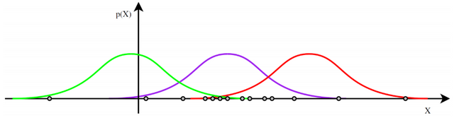
In the picture above, if one asks you “What is the Gaussian that has generated the samples?” you will probably answer the purple one. The real question is “Why is that one?". Let’s start by saying why the other two are not the ones you want. If we consider for example the last point on the left, it is very unlikely that it comes from the red distribution, since it is very far away from it, so the probability is basically zero. But I have observed this point…so probably the red option is not the right one! The same holds for the last point on the right, so we can infer that also the green one is not the true distribution. This is the idea behind Likelihood Estimation: I want to have a distribution for which I have at least some probability of observing the data. Wait, why not the maximum probability? From here, the Maximum Likelihood Estimation.

MLE is not the most probable model. We are not maximizing the likelihood of the model, we are maximizing the likelihood of the data.

MLE works as follows (note that it works also with other distributions):

Let $\theta = (\theta_1,\theta_2,…,\theta_p)^T$ a vector of parameters, find the MLE for $\theta$:

• Write the likelihood $L = P(Data|\theta)$ for the data
• (optional) Take the logarithm of likelihood $l = log P(Data|\theta)$
• Work out $\frac{\partial L}{\partial \theta}$ or $\frac{\partial l}{\partial \theta}$
• Solve $\frac{\partial L}{\partial \theta} = 0$ or $\frac{\partial l}{\partial \theta} = 0$
• Check that $\theta^{MLE}$ is a maximum

The ‘logarithm’ part is optional, but it is useful for two reasons:

• logarithms transform products into sums (we are interested in this)
• logarithms rescale the dynamic of the input

To maximize/minimize the (log)likelihood there are different ways, one of which is the Gradient Descent we mentioned before. In this case, however, we will use the exact solution.

Coming back to the i.i.d. samples we considered before, let’s apply the steps we listed above:

$$ L = P(Data|\theta) = p(x_1,x_2,…,x_N|\mu,\sigma^2) = \prod_{n=1}^{N} p(x_n|\mu,\sigma^2) = \prod_{n=1}^{N} \frac{1}{\sqrt{2\pi}\sigma} e^{-\frac{(x_n-\mu)^2}{2\sigma^2}} $$

$$ \displaylines{l = log P(Data|\theta) = log \Big( \prod_{n=1}^{N} \frac{1}{\sqrt{2\pi}\sigma} e^{-\frac{(x_n-\mu)^2}{2\sigma^2}} \Big) = \\ = \sum_{n=1}^{N} log \frac{1}{\sqrt{2\pi}\sigma} e^{-\frac{(x_n-\mu)^2}{2\sigma^2}} = \\ = N \cdot log \frac{1}{\sqrt{2\pi}\sigma} - \frac{1}{2\sigma^2} \sum_{n}^{N} (x_n - \mu)^2} $$

$$ \displaylines{\frac{\partial l(\mu)}{\partial \mu} = \frac{\partial}{\partial \mu} \Big( N \cdot log \frac{1}{\sqrt{2\pi}\sigma} - \frac{1}{2\sigma^2} \sum_{n}^{N} (x_n - \mu)^2 \Big) = \\ = -\frac{1}{2\sigma^2} \frac{\partial}{\partial \mu} \sum_{n}^{N} (x_n - \mu)^2 = -\frac{1}{2\sigma^2} \sum_{n}^{N} 2(x_n - \mu)} $$

$$ \displaylines{-\frac{1}{2\sigma^2} \sum_{n}^{N} 2(x_n - \mu) = 0 \\ \sum_{n}^{N} (x_n - \mu) = 0 \\ \sum_{n}^{N} x_n = \sum_{n}^{N} \mu \implies \mu_{MLE} = \frac{1}{N} \sum_{n}^{N} x_n} $$

Ok, good, so let’s now apply what we got to neural networks. Consider the regression problem: our goal is to approximate a target function $t$ having $N$ observations.

$$ t_n = g(x_n|w) + \epsilon_n, \quad \epsilon_n \sim N(0,\sigma^2) \implies t_n \sim N(g(x_n|w), \sigma^2) $$

Note that $t_n$ is a classical Gaussian, which has $g(x_n|w)$ instead of $\mu$. So let’s apply the MLE recipe:

$$ \displaylines{L(w) = p(t_1,t_2,…,t_N|g(x|w), \sigma^2) = \prod_{n=1}^{N} p(t_n|g(x_n|w),\sigma^2) = \\ = \prod_{n=1}^{N} \frac{1}{\sqrt{2\pi}\sigma} e^{-\frac{(t_n-g(x_n|w))^2}{2\sigma^2}}} $$

We look for weights which maximize the likelihood:

$$ \displaylines{argmax_w L(w) = argmax_w \prod_{n=1}^{N} \frac{1}{\sqrt{2\pi}\sigma} e^{-\frac{(t_n-g(x_n|w))^2}{2\sigma^2}} = \\ = argmax_w \sum_{n}^{N} log \Big( \frac{1}{\sqrt{2\pi}\sigma} e^{-\frac{(t_n-g(x_n|w))^2}{2\sigma^2}} \Big) = \\ = argmax_w \sum_{n}^{N} log \frac{1}{\sqrt{2\pi}\sigma} - \frac{1}{2\sigma^2} (t_n-g(x_n|w))^2 = \\ = argmin_w \sum_{n}^{N} (t_n-g(x_n|w))^2} $$

We finally reach the end. As you can see, under the assumptions we made for the regression case, in order to find the weights that maximize the likelihood we have to minimize exactly the sum of squared errors, our initial error function.

Observations:

• What if $t_n$ is not Gaussian? You can still do this, but it’s not the best solution, or at least it’s not a maximum likelihood estimation, so you can obtain a solution which is not unbiased.

• Can we derive something different knowing the errors are distributed differently? Well, if we know the distribution of the error yes, the only thing the we have to do is to follow the process we’ve seen, until we get to some result.

Regarding the second observation, if you think a bit, there is one common problem in which we know the distribution of $t_n$: binary classification.

$$ t_n \in {0,1} \implies t_n \sim Be(g(x_n|w)) $$

$$ p(t|g(x|w)) = g(x|w)^t \cdot (1-g(x|w))^{1-t} $$

where $t$ acts as a selector.

$$ \displaylines{L(w) = p(t_1,t_2,…,t_N|g(x|w)) = \prod_{n=1}^{N} p(t_n|g(x_n|w)) = \\ = \prod_{n=1}^{N} g(x_n|w)^{t_n} \cdot (1-g(x_n|w))^{1-t_n}} $$

$$ \displaylines{argmax_w L(w) = argmax_w \prod_{n=1}^{N} g(x_n|w)^{t_n} \cdot (1-g(x_n|w))^{1-t_n} = \\ = argmax_w \sum_{n}^{N} t_n log; g(x_n|w) + (1-t_n) log (1-g(x_n|w)) = \\ = argmin_w -\sum_{n}^{N} t_n log; g(x_n|w) + (1-t_n) log (1-g(x_n|w))} $$

We have obtained a new error function, called cross-entropy error function. Why is it different from the one we found before? Because they solve different problems: regression (additive Gaussian noise), classification (predictive Bernoulli distribution). Basically, the error function that you are minimizing describes the problem you’re trying to solve. If so, how can we design a new error function?

• Use all your knowledge/assumptions about the data distribution
• Exploit background knowledge on the task and the model
• Use your creativity (lots of trial and error)

Final Comments

Let’s make a final observation considering the following samples:

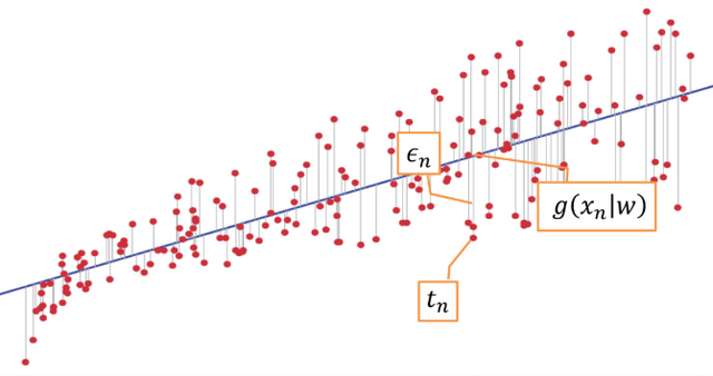
By looking at this data, I immediately observe that the hypothesis that they come from a nonlinear function plus a Gaussian noise with some constant variance is wrong. Indeed, the dispersion of points is different; more precisely, when the value we want to predict is small, the error is small, and when the value we want to predict is high, the error is high. There is a correlation between the noise and the function we want to learn, and this correlation is not described in the squared error function. The hypothesis of constant variance in the data is called homoscedasticity, which in this case is not true. Thus, there might be a better error function to deal with this data, which takes into consideration the so called eteroscedasticity. Another way to see the problem is that when you have to draw the line which represents your model, you will give more importance to the last samples, not because they are more important, but because in those points the error is bigger. This was just to say that in some cases the squared error function is not enough and you have to apply some changes.

Just to conclude, to handle the case of the picture, we can think to have something like:

$$ t_n = g(x_n|w) \cdot \epsilon_n $$

One trick that we can use in this scenario, which statisticians call variance stabilizing transformation, is to make the regression of $log t$, instead of the regression of $t$:

$$ log t_n = log(g(x_n|w)) + log(\epsilon_n) $$

If the effect of distorsion of the variance is not too big, this method can sometimes solve the problem. There are other transformations, like sqrt, polynomial etc.