In this post I will explain Image Segmentation, focusing on the architecture of the models used to perform this task. Fully Convolutional Networks and U-Net will be at the center of the discussion.
Disclaimer: These notes are for the most part a collection of concepts taken from the slides of the ‘Artificial Neural Networks and Deep Learning’ course at Polytechnic of Milan and from some other online resources. I am just putting together all the information to study for the exam and I thought it would be a good idea to upload them here since they can be useful for someone interested in this topic.
Image Segmentation
In the last post, we introduced CNNs and their use in image classification. Image segmentation is not so different, that’s why I suggest you to read the ‘Introduction to CNN’ first if you haven’t already done it.
Indeed, if in image classification we want to assign a label to a whole image, in image segmentation we want to assign a label to every pixel in an image such that pixels with the same label share certain visual characteristics.
Fully Convolutional Networks
Paper: Fully Convolutional Networks for Semantic Segmentation
In order to understand the differences between a CNN and a FCN let’s analyze the architectures:
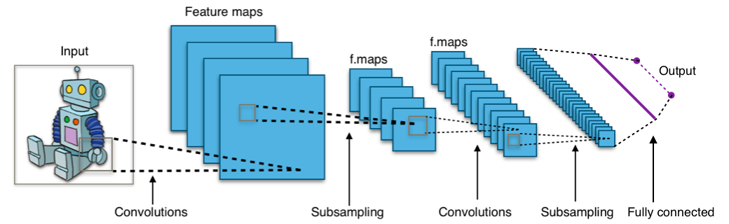
As we can see from the above image, a typical CNN can be seen as a stack of convolutional and pooling layers, ended by a fully connected layer, which is a standard Multi-Layer Perceptron. With an architecture like this, if we feed an input image with a larger size w.r.t. the one used for the training, the model would not work, because even if the convolutional part is size independent, the final fully connnected layer has a fixed input size.
However, the FC is linear, so it can be represented as a convolution. More precisely, citing the paper:
The fully connected layers of these nets have fixed dimensions and throw away spatial coordinates. However, these fully connected layers can also be viewed as convolutions with kernels that cover their entire input regions. Doing so casts them into fully convolutional networks that take input of any size and output classification maps.
Fully Convolutional Networks for Semantic Segmentation
So, assuming to have a fully connected layer like this:
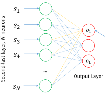
this can be represented as a 2D convolutional layer against $L$ filters having size $1 \times 1 \times N$.
Ok, but what do we obtain as output now? Well, for each output class we obtain an image having lower resolution than the input image and class probabilities for the receptive field of each pixel: heatmaps.
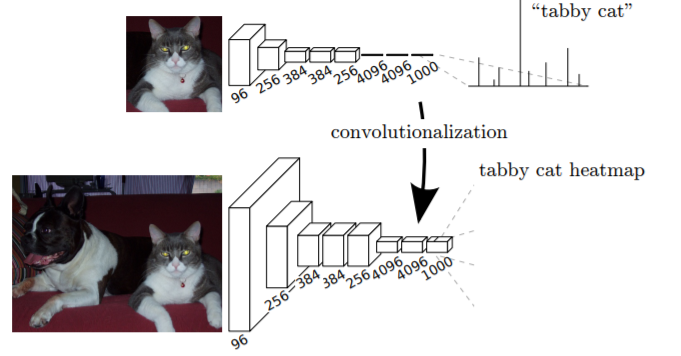
Image from the paper Fully Convolutional Networks for Semantic Segmentation
Consider for example the heatmap that corresponds to the “wheel” class: it’s telling us how much likely in the receptive field associated to this pixel there is something that looks like a wheel.
Approaches to segmentation
Direct heatmap predictions
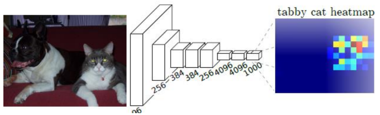
Image from the paper Fully Convolutional Networks for Semantic Segmentation
The idea here is that we can take the last volume in the network, which is the output of our CNN, having depth 1000. We slice this volume 1000 times and for each slice, namely for each class, we take the argmax, through which we obtain an image that contains in each pixel the index of the slice referring to the most probable class. What’s the drawback of this approach? It is a very coarse estimate, since going through the convolution we are losing a lot of spatial resolution.
The shift and stitch
As we have seen, mapping the output directly to the input will cause resolution to look patchy. The idea behind the shift and stitch method is to take the same input and to shift it a bit multiple times, computing a heatmap for all $f^2$ possible shifts. We then map predictions from the heatmaps to the image (each pixel in the heatmap provides prediction of the central pixel of the receptive field). Finally, we interleave the heatmaps to form an image as large as the input.
One might think of it as taking multiple (shifted) low resolution images of an object and combining (stitch) them to get a higher resolution image.
I found an image from this website which can help to get the idea:
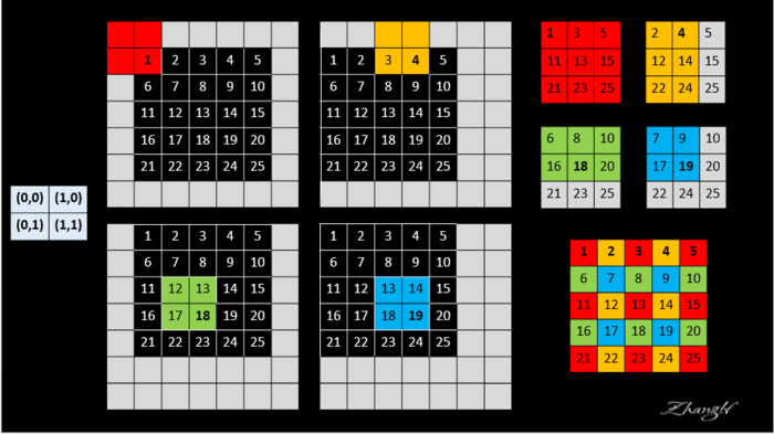
Assume that your FCN is a $2 \times 2$ max pooling layer. Every time the input (the black pixels) is shifted, you obtain a different heatmap ($3 \times 3$). At the end, you take all the heatmaps and you stitch them together.
Although performing this transformation naively increases the cost by a factor of $f^2$, there is an efficient implementation through the à trous algorithm. However, the upsampling part is very rigid: we would like to learn also this part.
Only convolutions
Another approach would be that of using only convolutional and activation layers, without any subsampling. Two problems:
- very small receptive field
- very inefficient, since convolutions at original image resolution will be very expensive
Upsampling
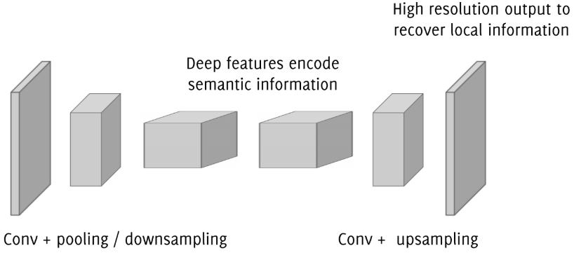
Ok, so what can we do? There is a clear tradeoff here: on the one hand we need to go deep to extract high level information on the image, on the other hand we want to stay local to not lose spatial resolution in the prediction.
Semantic segmentation faces an inherent tension between semantics and location:
- global information resolves what
- local information resolves where
The good news is that upsampling filters can be learned during training, since linear upsampling of a factor $f$ can be implemented as a convolution against a filter with a fractional stride $1/f$.
CS231n: Convolutional Neural Networks for Visual Recognition
CS231n: Convolutional Neural Networks for Visual Recognition
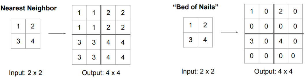
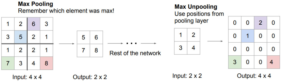
One problem with these three approaches is that there are no parameters, so they are not learnable. Let’s see something that is learnable.
Transpose convolution
With transpose convolution we’re changing the role of the filter. Indeed, suppose for example to have an input image of size $5 \times 5 \times 1$ and a filter of size $3 \times 3 \times 1$ with stride $2 \times 2$ and padding VALID. The output will be a $2 \times 2$ image.
Ok, now we want to upsample this output to the original image. In order to do so, by using the same filter of size $3 \times 3$, we multiply each value of our $2 \times 2$ image with the values of the filter. This procedure is repeated for each pixel of the input image, moving the filter according to the stride (2 in our example).
CS231n: Convolutional Neural Networks for Visual Recognition
Skip connections
Nice, so we have finished! Not really, these are the results obtained by the authors of the paper:
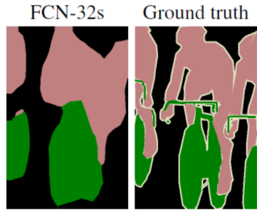
Image from the paper Fully Convolutional Networks for Semantic Segmentation
Where 32 is the number of times the image has been upsampled.
As we can see, the result is not very good. This means that this upsampling is not able to recover all the spatial information. Where can we grab this information? We need higher resolution information about the content of the image, so a good starting point would be to go in the shallow layers. This is the reason for which skip connections were introduced.
Combining fine layers and coarse layers lets the model make local predictions that respect global structure.
Fully Convolutional Networks for Semantic Segmentation
The idea is to combine the upsampled output of one layer in the upsampling part of the network with the unchanged output of a previous layer in the downsampling part of the network by adding them together. The result of this sum will be upsampled again and summed with a shallower layer in the downsampling part, and so on.
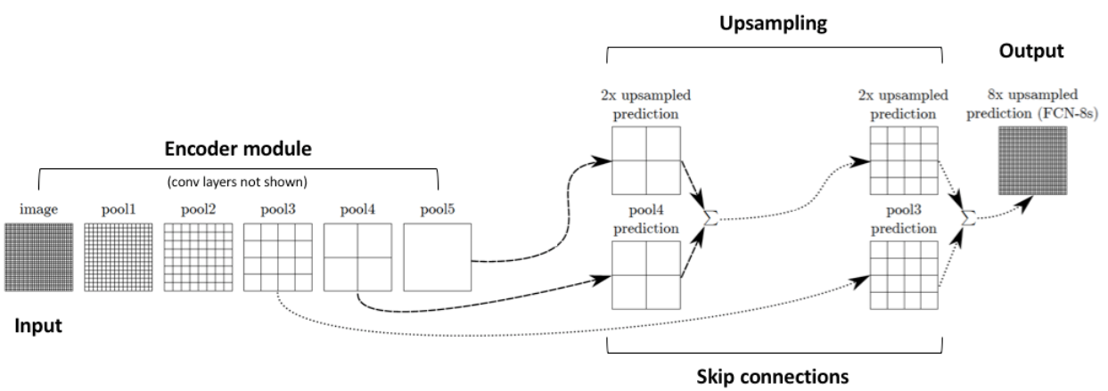
https://www.jeremyjordan.me/semantic-segmentation/
As written in the paper, this process yields 3 models:
- Train first the lowest resolution network (FCN-32s)
- Then the weights of the next network (FCN-16s) are initialized with (FCN-32s)
- The same for FCN-8s
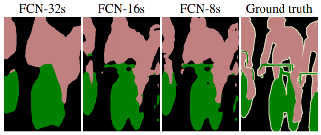
Image from the paper Fully Convolutional Networks for Semantic Segmentation
Training a F-CNN (and segmentation networks)
Patch-based way
- Prepare a training set for a classification network
- Crop as many patches from annotated images and assign to each patch label corresponding to the patch center
- Train a CNN for classification from scratches, or fine-tune a pre-trained model over the segmentation classes
- Once trained the network, move the FC layers to $1 \times 1$ convolutions
- Train the upsampling filters
The classification network is trained to minimize the classification loss $l$ over a mini-batch:
$$ \hat{\theta} = min_{\theta} \sum_{\boldsymbol{x_j}} l(\boldsymbol{x_j},\theta) $$
where $\boldsymbol{x_j}$ belongs to a mini-batch.
Batches of patches are randomly assembled during training and it is possible to resample patches for solving class imbalance. However, this approach is very inefficient, since convolutions on overlapping patches are repeated multiple times.
Full-image way
$$ \hat{\theta} = min_{\theta} \sum_{\boldsymbol{x_j}} l(\boldsymbol{x_j},\theta) $$
The loss function is the same, but in this case $\boldsymbol{x_j}$ are all the pixels in a region of the input image and the loss is evaluated over the corresponding labels.
In the previous approach if you want to classify a whole image you have to crop multiple patches, so if you have input images of size $500 \times 500$ and you train your network to classify patches of size $90 \times 90$ to recover the value of the label which is in the central pixel. This means that in practice you have to compute the same convolution multiple times.
Instead, if you directly train your network in order to perform segmentation and to provide as output the image of the labels, and if you compute the loss by comparing the output labels with the ground truth, you have to compute convolution only once, because you’re moving the whole image through the network.
The drawback of the full-image approach, however, is that we are losing the randomness of the minibatches which is present in the patch-based way (due to the fact they can be randomly selected). Although, we can recover this randomness to make the estimated loss a bit stochastic by using some random masks, excluding some pixels when computing the loss:
$$ minimize \sum_{\boldsymbol{x_j}} M(\boldsymbol{x_j}) l(\boldsymbol{x_j},\theta) $$
being $M(\boldsymbol{x_j})$ a binary random variable.
Another problem is the class imbalance. With patch-wise training this is not a problem, since we can repeat the same patch multiple times to adjust the difference in terms of number of samples. Instead, with full-image approach this is not possible. Also in this case we can compensate by weighting the loss:
$$ minimize \sum_{\boldsymbol{x_j}} w(\boldsymbol{x_j}) l(\boldsymbol{x_j},\theta) $$
being $w(\boldsymbol{x_j})$ a weight that takes into account the true label of $\boldsymbol{x_j}$.
U-Net
Paper: U-Net: Convolutional Networks for Biomedical Image Segmentation
This paper was published in the same period of time as the previous one, although this seems to be a bit more famous. The concepts behind the architecture of this model are exactly the ones we’ve discussed so far. However, there are some interesting details.
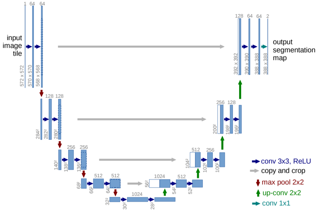
Image from the paper U-Net: Convolutional Networks for Biomedical Image Segmentation
It is pretty obvious the reason for which it was called U-Net.
The contracting path follows the typical architecture of a convolutional network. It consists of the repeated application of two 3x3 convolutions (unpadded convolutions), each followed by a rectified linear unit (ReLU) and a 2x2 max pooling operation with stride 2 for downsampling. At each downsampling step we double the number of feature channels. Every step in the expansive path consists of an upsampling of the feature map followed by a 2x2 convolution (“up-convolution”) that halves the number of feature channels, a concatenation with the correspondingly cropped feature map from the contracting path, and two 3x3 convolutions, each followed by a ReLU. The cropping is necessary due to the loss of border pixels in every convolution. At the final layer a 1x1 convolution is used to map each 64-component feature vector to the desired number of classes. In total the network has 23 convolutional layers.
U-Net: Convolutional Networks for Biomedical Image Segmentation
Note indeed that a major difference w.r.t. (long et al. 2015) is that U-Net uses a large number of feature channels in the upsampling part, leading the network to become symmetric.
Another interesting detail is how the information coming from the skip connections are combined with the one coming from the upsampling path: they are concatenated and then mixed in a learnable manner through convolution.
Training
The network was trained using a full-image approach with the following weighted loss function:
$$ \hat{\theta} = min_{\theta} \sum_{\boldsymbol{x_j}} w(\boldsymbol{x_j}) l(\boldsymbol{x_j},\theta) $$
where the weight
$$ w(\boldsymbol{x}) = w_c(\boldsymbol{x}) + w_0 e^{-\frac{(d_1(\boldsymbol{x}) + d_2(\boldsymbol{x}))^2}{2\sigma^2}} $$
- $w_c$ is used to balance class proportions (since it’s a full-image approach)
- $d_1$ is the distance to the border of the closest cell
- $d_2$ is the distance to the border of the second closest cell
The second term is indeed used to enhance classification performance at borders of different objects, that in the scenario in which this network was used by the authors of the paper was very useful.
Data augmentation
An interesting fact is that if in the first paper the authors said that data augmentation
yielded no noticeable improvement
In the U-Net paper, instead, they claim that data augmentation
is essential to teach the network the desired invariance and robustness properties, when only few training samples are available. […] Especially random elastic deformations of the training samples seem to be the key concept to train a segmentation network with very few annotated images.
Indeed, the two scenario are pretty different, so as always data augmentation must be performed according to the problem we’re facing.