In this post I will give you an introduction to Convolutional Neural Networks (CNN). We will see the reasons behind the success of this architecture and the latter will be analyzed layer by layer.
Disclaimer: These notes are for the most part a collection of concepts taken from the slides of the ‘Artificial Neural Networks and Deep Learning’ course at Polytechnic of Milan, the book ‘Deep Learning’ (Goodfellow-et-al-2016) and from some other online resources. I am simply putting together all the information to study for the exam and I thought it would be a good idea to upload them here since they can be useful for someone who is interested in this topic.
Introduction to CNN
The convolution operation
Convolution is a mathematical operation on two functions ($f$ and $g$) that produces a third function expressing how the shape of one is modified by the other. The term convolution refers to both the result function and to the process of computing it.
The convolution of $f$ and $g$ is written $f∗g$ and it can be computed as follows:
$$
s(t) = (f∗g)(t) = \int_{-\infty}^\infty f(\tau) g(t-\tau) d\tau
$$
In convolutional network terminology, the first argument (in this case the function $f$) is called input and the second argument (in this case the function $g$) is called kernel. The output is usually referred to as the feature map.
Of course, since we work with computers time will be discretized, thus we can define the discrete convolution:
$$
s(t) = (f∗g)(t) = \sum_{a = -\infty}^\infty f(a) g(t-a)
$$
We often use convolutions over more than one axis at a time. For example, if we use a two-dimensional image $I$ as input, we probably also want to use a two-dimensional kernel $K$:
$$ S(i,j) = (I∗K)(i,j) = \sum_m \sum_n I(m,n)K(i-m,j-n) $$
or, since convolution is commutative:
$$ S(i,j) = (K∗I)(i,j) = \sum_m \sum_n I(i-m,j-n)K(m,n) $$
Note that what is actually implemented in many neural network libraries is the cross-correlation function, which is the same as convolution but without flipping the kernel:
$$ S(i,j) = (I∗K)(i,j) = \sum_m \sum_n I(i+m,j+n)K(m,n) $$
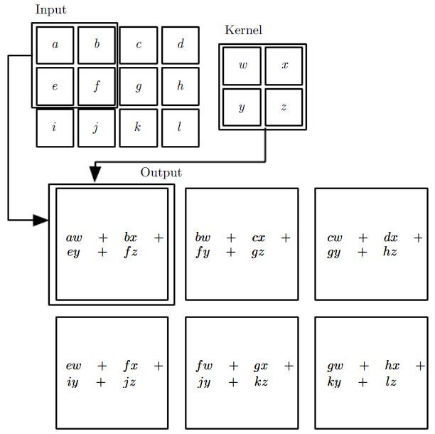
Image from the Deep Learning boox
Image Classification: the problem
Given an input image $I$, assign a label $l$ from a fixed set of categories.
Challenges in image classification:
- Images are very high-dimensional data. The CIFAR10 dataset, for example, has very small images (32x32) but still $d = 32 \times 32 \times 3 = 3072$
- Label ambiguity: a label might not uniquely identify an image
- Transformations: there are many transformations that change the image dramatically, but not its label
- Inter-class variability: images in the same class might be dramatically different
- Perceptual similarity: perceptual similarity is not related to pixel similarity. This is the reason for which if we use a Nearest Neighborhood Classifier, assigning to each test image the label of the closest image in the training set, the results will be bad.
Linear Classifier
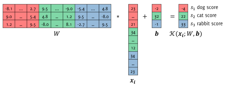
where $W$ are the weights, $\boldsymbol{b}$ is the bias (both parameters of the classifier $K$), and $\boldsymbol{x_i}$ is our unrolled image.
$$ K(\boldsymbol{x}) = W\boldsymbol{x} + \boldsymbol{b} $$
The classifier assigns to an input image the class corresponding to the largest score:
$$ \hat{y}_j = \underset{i=1…L}{\operatorname{argmax}} [s_j]_i $$
being $[s_j]_i$ the i-th component of the vector $K(\boldsymbol{x_j}) = W\boldsymbol{x_j} + \boldsymbol{b}$.
As said before, $W$ and $\boldsymbol{b}$ are parameters of the classifier. They are defined by training our classifier in order to minimize some loss function over a whole training set TR:
$$ [W,b] = argmin_{W \in R^{L \times d}, b \in R^L} \sum_{(x_i,y_i) \in TR} L(x,y_i) $$
Denoting $W(i,:)$ as the d-dimensional vector containing the weights of the score function for the i-th class, it can be seen as a template used in matching.
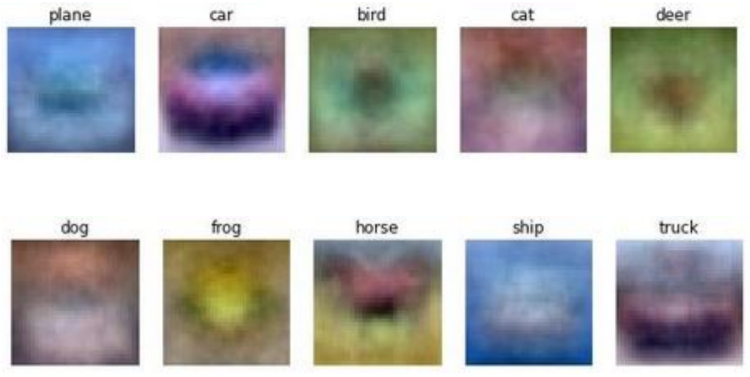
Templates learned on the CIFAR10 dataset
As we can see the model has learned that the background of planes and boats is blue, that cars are typically red and so on. It is definitely too simple to achieve higher performance and better templates. We thus need a better approach.
Feature Extraction
Probably, feeding the images directly to the classifier is not a good idea. We need some intermediate steps with which we can extract meaningful information and also reduce the data-dimension.
Of course, these features can be hand-crafted according to the problem we are facing. However, this is in general not advisable, since usually the patterns are very complex, there are many variables and there is a high risk of overfitting. As we know, neural networks are instead a good tool in this scenario, thanks to the fact that deep learning techniques are able to independently learn a hierarchical set of meaningful features.
Convolutional Neural Networks
CNN are typically made of blocks that include:
- convolutional layers
- nonlinearities (activation functions)
- pooling layers (usually max pooling)
First of all, why convolution? There are 3 main reasons:
-
sparse connectivity: In traditional neural networks every output unit interacts with every input unit (fully connected). This does not happen in CNN, where we typically have sparse interactions (or sparse weights). This is accomplished by making the kernel smaller than the input. This is particularly important with images, since as we said we have to deal with high-dimensional data. This approach, indeed, means that we need to store fewer parameters, which both reduces the memory requirements of the model and improves its statistical efficiency. Moreover, it also means that computing the output requires fewer operations.
-
parameter sharing: In a traditional neural network, each element of the weight matrix is used exactly once when computing the output of a layer. In a CNN, each member of the kernel is used at every position of the input (except perhaps some of the boundary pixels, we will see more on this later). This means that rather than learning a separate set of parameters for every location, we learn only one set. This further reduces the storage requirements of the model to $k$ parameters.
-
equivariant representations: thanks to parameter sharing, layers in CNN have a property called equivariance to translation. We say that a function is equivariant when if the input changes, the output changes in the same way. With images, convolution creates a 2D map of where certain features appear in the input. If we move the object in the input, its representation will move the same amount in the output. A very good explanation of this property can be found HERE.
CNN Architecture
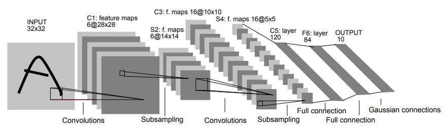
LeCun, Yann, et al. "Gradient-based learning applied to document recognition" (1998)
The above architecture is the LeNet-5, a pioneering 7-level convolutional network by LeCun et al. in 1998, that classifies digits (http://yann.lecun.com/exdb/lenet/).
Let’s analyze it.
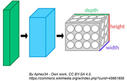
- An image passing through a CNN is transformed in a sequence of volumes
- As the depth increases, the height and width of the volume decreases
- Each layer takes as input and returns a volume
Convolutional layer
As we have already seen, the convolutional layers consists of a linear combination of all the values in a region of the input. The parameters of this layer are called filters or kernels, and they represent the weights of the linear combination. During training, a CNN finds the most useful filters for its task, and it learns how to combine them into more complex patterns.
If we assume for example to have an input image with size $32 \times 32 \times 3$ (depth 3 in case of RGB image), we can use for example a filter $3 \times 3 \times 3$ in order to compute convolution (note that the depth of the filter must be the same as the depth of the image). This means that our filter will move over the image and at each step we obtain 3 values, one for each level of the input. These values will be summed together and then with the bias, in order to obtain a single value, that will be part of the resulting feature map.
Visualizing what just described:
Credits: Towards Data Science - A Comprehensive Guide to Convolutional Neural Networks
Two things to notice from the above image:
- There are some zeros in the border of the image. The reason is that in order for a layer to have the same height and width as the previous layer, it is common to add zeros around the input (zero padding).
- The filter shifts of 1 pixel at a time. This value can be set and it’s called stride, which indeed represents the distance between two consecutive receptive fields.
Moreover, note that in this representation the volume of the output has not increased. This is due to the fact that we used only one filter.
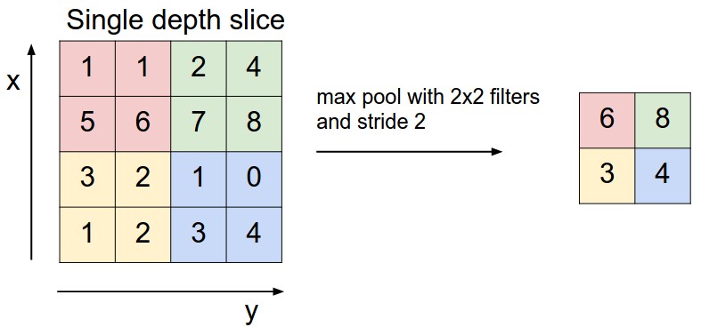
Pooling layer
The goal of pooling layers is pretty simple: reduce the spatial size of the volume. This is done by subsampling the input image, usually using the MAX operation. In addition to reducing the computational load, the memory usage and the number of parameters, pooling also makes neural networks a bit more tolerant with respect to image shift, which can greatly improve the statistical efficiency of the network under the assumption that the function that the layer learns is invariant to small translations. Also in this layer we can define the size and the stride.
And then?
More or less we are done. The basic CNN architecture is simply a stack of convolutional layers (each one followed by an activation function) and pooling layers (usually max pooling). Going through this pipeline, the image generally gets smaller and smaller, but deeper and deeper (more and more feature maps). At the end of this stack there is a standard feedforward neural network, with some fully connected layers and generally a final softmax layer, providing as output class probabilities.
With some changes, but this is exactly the architecture of LeNet-5, that we saw before. In the last years, many variants have been developed, like AlexNet, GoogLeNet, ResNet etc., which I will not explain here (maybe in future dedicated posts).
The receptive field
More or less, we have already talked about the receptive field, but let’s add some useful insights. It’s interesting to know that concept of receptive field comes from an experiment on cats and then monkeys carried out by David H. Hubel and Torsten Wiesel (who received the Nobel prize for their work).
They showed that many neurons in the visual cortex have a small local receptive field, meaning they react only to visual stimuli located in a limited region of the visual field. Moreover, the authors showed that some neurons react only to images of horizontal lines, while others react only to lines with different orientations. They also noticed that some neurons have larger receptive fields, and they react to more complex patterns that are combinations of the lower-level patterns.
Hands-On Machine Learning (1st edition) - Aurélien Géron
We can now well understand what is the idea behind CNN. As we said, unlike in fully connected layers, where the value of each output depends on the entire input, in CNNs an output only depends on a region of the input, the receptive field, precisely. The deeper you go, the wider the receptive field: convolution, max pooling and stride greater than 1 all increase the receptive field.
Conclusions
Much more can be said about CNNs, but since this is thought to be an intro to the topic I will stop here, leaving further details to the future.