In this post I will give you an introduction to Generative Adversarial Networks, explaining the reasons behind their architecture and how they are trained.
Disclaimer: These notes are for the most part a collection of concepts taken from the slides of the ‘Artificial Neural Networks and Deep Learning’ course at Polytechnic of Milan, the book ‘Deep Learning’ (Goodfellow-et-al-2016) and from some other online resources. I am simply putting together all the information to study for the exam and I thought it would be a good idea to upload them here since they can be useful for someone who is interested in this topic.
Generative Models
As the name suggests, generative models are models with the goal of generating new data instances. The adjective “generative” describes a class of statistical models that contrasts with discriminative models.
Generative models, indeed, capture the joint probability $P(X,Y)$, telling us how likely a given example is, while discriminative models capture the conditional probability $P(Y | X)$, ignoring how likely a given example is and just telling how likely a label is to apply to the instance.
Autoencoders as generative models
I will assume that autoencoders are a familiar architecture to the reader, and in the future I’ll probably write a specific post about them. In the meanwhile, it is enough to know that an autoencoder is a specific type of neural network, which is trained to attempt to copy its input to its output. Even if it can sound strange, these models are very useful, since they allow to have an internal and lower-dimension representation of the input data. In fact, the original use of autoencoders was dimensionality reduction and feature learning.
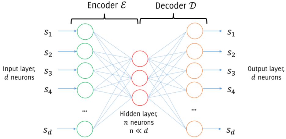
In recent years, autoencoders have started to be used also as generative models. The idea is the following:
- Train an autoencoder on a training set of images $S$
- Discard the encoder
- Draw random vectors to replace the latent representation and feed this to the decoder input
The problem of this approach is that we don’t know the distribution of proper latent representation, or at least it is very difficult to estimate.
Generative Adversarial Networks (GANs)
Reference paper: Generative Adversarial Nets
The difference w.r.t. the previous approach is that here we do not look for an explicit density model describing the manifold of natural images, but we just find out a model that is able to generate samples that “look like” our training samples.
Now, the main challenge is: how can we define a suitable loss?
The idea is to adopt a game theoretic scenario in which the generator network must compete against an adversary. The generator network tries to produce realistic samples in order to fool the discriminator network. The discriminator network tries to distinguish between samples drawn from the training data and samples drawn from the generator, emitting a probability value indicating that $\boldsymbol{x}$ is a real training example.
Thus, we train both networks and once finished, the decoder can be discarded (since it will output $\frac{1}{2}$ everywhere).
Considering that
- the samples produced by the generator are $\boldsymbol{x} = g(\boldsymbol{z};\boldsymbol{\theta}^{(g)})$
- the emitted probability value of the discriminator is $d(\boldsymbol{x};\boldsymbol{\theta}^{(d)})$
- the payoff received by the discriminator is $v(\boldsymbol{\theta}^{(g)}, \boldsymbol{\theta}^{(d)})$
- the payoff received by the generator is $-v(\boldsymbol{\theta}^{(g)}, \boldsymbol{\theta}^{(d)})$
Since during learning both the generator and the discriminator attempt to maximize its own payoff:
$$
g^* = arg\; min_g\; max_d\; v(g,d)
$$
where
$$ v(\boldsymbol{\theta}^{(g)}, \boldsymbol{\theta}^{(d)}) = E_{\boldsymbol{x} \sim p_{data}} log; d(\boldsymbol{x}) + E_{\boldsymbol{x} \sim p_{model}} log(1 - d(\boldsymbol{x})) $$
Training
Because of the particular structure of a GAN, where we have two different trained networks, two problems arise when training:
- two different kinds of training (generator and discriminator)
- convergence is hard to identify
Alternate training
The idea is to train the two networks in separated periods:
- Train the discriminator for one or more epochs. During these steps, the generator is kept constant, because the discriminator has to learn the imperfections of the generator, and of course a trained generator is different from a generator that produces random outputs, as happens at the beginning.
- Train the generator for one or more epochs. During these steps, the discriminator is kept constant, otherwise the generator should try to hit a moving target and might not converge.
- Repeat
As said, convergence is also a problem, since the discriminator feedback gets less meaningful over time and if the GAN is trained after the point in which the discriminator gives as output a $\frac{1}{2}$ probability, the generator would start to train on junk feedback.
Image from Generative Adversarial Nets
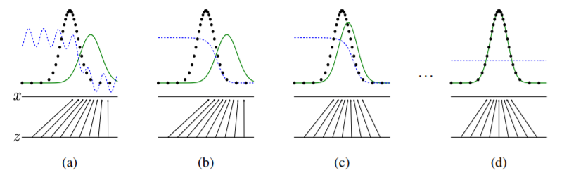
Image from Generative Adversarial Nets
I think the above image is very interesting and helps to understand what is going on during the training procedure: the lowest line is the domain from which $\boldsymbol{z}$ is sampled, while the above one is part of the domain of $\boldsymbol{x}$. The arrows represent the mapping $g(\boldsymbol{z};\boldsymbol{\theta}^{(g)})$, and in fact one can see that the green line, i.e. the generative distribution, is positioned according to them. Instead, the black dotted line represents the data generating distribution, and the blue one the discriminative distribution. The latter is positioned according to its emitted probability, and we can see that on the left of each plot the probabilities are high, since the samples are real training examples, while on the right it correctly recognizes the fake ones produced by the generator. During training we can see how the generator shifts its generative distribution to match the data distribution and how the discriminator struggles to discriminate between fake and real, until reaching convergence, i.e. the horizontal line at probability $\frac{1}{2}$.
Improvements over the years
If you are interested, these are some papers that improved the original GAN:
- Unsupervised Representation Learning With Deep Convolutional Generative Adversarial Networks
- Progressive Growing of GANs for Improved Quality, Stability, and Variation
- Wasserstein GAN
- Unpaired Image-to-Image Translation using Cycle-Consistent Adversarial Networks
- Self-Attention Generative Adversarial Networks