In this post I will go through Recurrent Neural Networks (RNNs) and Long-Short Term Memories (LSTMs), explaining why RNNs are not enough to deal with sequence modeling and how LSTMs solve those problems.
Disclaimer: These notes are for the most part a collection of concepts taken from the slides of the ‘Artificial Neural Networks and Deep Learning’ course at Polytechnic of Milan, the book ‘Deep Learning’ (Goodfellow-et-al-2016) and from some other online resources. I am simply putting together all the information to study for the exam and I thought it would be a good idea to upload them here since they can be useful for someone who is interested in this topic.
Sequence Modeling
So far we have considered only “static” datasets, i.e. datasets where the time component is not present. However, we know that there are problems in which time cannot be ignored, like in the case we want to predict the next word given one or more previous words. Sequence modeling is the task of predicting what comes next, and to do this the current output must depend on the previous input and the length of the input is not fixed.
There exist different ways to deal with “dynamic” data:
- Memoryless models
- Autoregressive models
- Feedforward Neural Networks
- Models with memory
- Linear dynamical systems
- Hidden Markov Models
- Recurrent Neural Networks
- …
We will focus on Recurrent Neural Networks (RNNs).
Recurrent Neural Networks (RNNs)
Much as convolutional neural networks are neural networks specialized for processing a grid of values like an image, recurrent neural networks are neural networks specialized for processing a sequence of values.
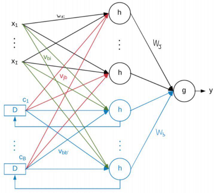
The blue part in the above image is the so-called context network. In the context network new neurons are added in the hidden layer and their output is not only connected to the output layer, but it is also delayed and connected again to the hidden layer (in the following time step).
$$ y^t = g(\sum_{j}^{J} W_j \cdot h(\sum_{i}^{I} w_{ji} \cdot x_i^t + \sum_{b}^{B} v_{jb} \cdot c_b^{t-1}) + \sum_{b}^{B} W_b + h(\sum_{i}^{I} v_{bi} \cdot x_i^t + \sum_{b’}^{B} v_{bb’} \cdot c_{b’}^{t-1})) $$
$$ c_b^t = h(\sum_{i}^{I} v_{bi} \cdot x_i^t + \sum_{b’}^{B} v_{bb’} \cdot c_{b’}^{t-1}) $$
But how do we train this neural network? Because of the context network, we cannot use backpropagation anymore. However, we can see the context network as a feedforward neural network, if we unroll it.
Backpropagation Through Time
Backpropagation Through Time is the way in which we can train our RNN. As said, the idea is the following:
- Perform network unroll for $U$ steps
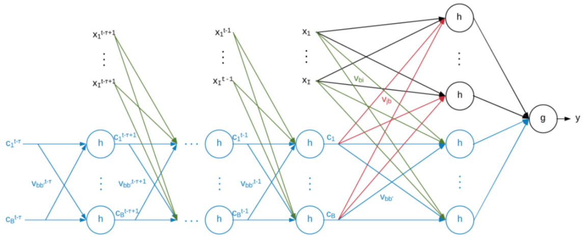
- All the weights are trained with gradient descent, so at a generic time step $\tau$:
$$ v_{bi}^{t-\tau} = v_{bi}^{t-\tau} - \eta \frac{\partial E}{\partial v_{bi}^{t-\tau}} $$
$$ v_{bb’}^{t-\tau} = v_{bb’}^{t-\tau} - \eta \frac{\partial E}{\partial v_{bb’}^{t-\tau}} $$
$$ v_{jb}^{t-\tau} = v_{jb}^{t-\tau} - \eta \frac{\partial E}{\partial v_{jb}^{t-\tau}} $$
- Average the weights, since if we apply the usual update method we would have different values for the same weights in different time steps.
$$ v_{bi} = \frac{1}{U + 1} \sum_{\tau=0}^{U} v_{bi}^{t-\tau} $$
$$ v_{bb’} = \frac{1}{U + 1} \sum_{\tau=0}^{U} v_{bb’}^{t-\tau} $$
$$ v_{jb} = \frac{1}{U + 1} \sum_{\tau=0}^{U} v_{jb}^{t-\tau} $$
Vanishing Gradient
We said that we unroll the network for $U$ steps, but how do we set this value? How much can we go back in time?
The answer is: not too much, and this is the biggest problem of RNNs.
Let’s consider a simplified case in order to better understand why it does not work:
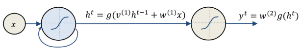
Backpropagation over an entire sequence is computed as
$$ \frac{\partial E}{\partial w} = \sum_{t=1}^{S} \frac{\partial E^t}{\partial w} $$
$$ \frac{\partial E^t}{\partial w} = \sum_{t=1}^{t} \frac{\partial E^t}{\partial y^t} \frac{\partial y^t}{\partial h^t} \frac{\partial h^t}{\partial h^k} \frac{\partial h^k}{\partial w} $$
$$ \frac{\partial h^t}{\partial h^k} = \prod_{i=k+1}^{t} \frac{\partial h_i}{\partial h_{i-1}} = \prod_{i=k+1}^{t} v^{(1)} g’(h^{i-1}) $$
If we consider the norm of these terms
$$ \Big|\Big|\frac{\partial h_i}{\partial h_{i-1}}\Big|\Big| = ||v^{(1)}|| ||g’(h^{i-1})|| \implies \Big|\Big|\frac{\partial h^t}{\partial h^k}\Big|\Big| \le (\gamma_v \cdot \gamma_{g’})^{t-k} $$
The key point is that if $(\gamma_v \cdot \gamma_{g’}) < 1$ the whole derivative converges to 0. This problem is called vanishing gradient, because as the gradient propagates over many stages it tends to vanish. There is also the opposite case, in which the gradient explodes, when $(\gamma_v \cdot \gamma_{g’}) > 1$, even if it is more rare.
This is a serious problem, because it essentially prevents our RNN to learn long-term dependencies (actually not very long, even with a 10-20 steps the problem can arise). This is especially true if we have sigmoid or tanh as activation functions, since they have a derivative smaller than $1$.
That is why a different activation function is used: the ReLU. We already discussed about ReLU in the post about activation functions, but the idea is pretty simple: it has derivative equal to $1$ for $x > 0$ and equal to $0$ for $x < 0$. This means that in the first case the gradient is propagated as it is, while in the second case it is not propagated at all. The latter fact, however, has a disadvantage: if the weights learned are such that $x < 0$ for the entire input domain, the neuron never learns: this problem is known as dying neuron. In order to solve this issue, Leaky ReLU was invented.
Another approach used to combat the vanishing gradient problem is the use of Leaky Units, i.e. hidden units with linear self-connections. The use of a linear self-connection with a weight near $1$ is a way of ensuring that the unit can access values from the past. These units allow the network to accumulate information over a long duration. However, it could be useful for the network to forget an old state and what we would like to do is to not set this behaviour manually, but instead let the network learn to decide when to do it. This brings us to the next model.
Long-Short Term Memories (LSTMs)
Original paper: LSTM Can Solve Hard Long Time Lag Problems
In 1997 Hochreiter and Schmidhuber published a paper in which they proposed a new model that is able to deal with long sequences without incurring in the vanishing gradient problem.
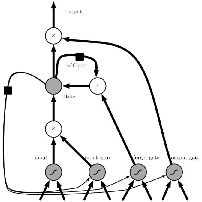
Image from http://www.deeplearningbook.org/
There are many artistic and cool images out there, but I found this very intuitive and useful to understand how a LSTM cell works. The important things to notice are:
- cells are connected recurrently to each other, replacing the standard hidden units
- the input value can be accumulated into the state if the sigmoidal input gate allows it
- the state unit has a linear self-loop (similar to the leaky units we discussed before) whose weight is controlled by the forget gate
- the output of the cell can be shut off by the output gate
- the state unit can also be used as an extra input to the gating units
- the black square indicates a delay of a single time step
RNNs vs LSTMs
Important: from now on I will base my notes on the post on LSTMs written by Christopher Olah, which I highly recommend to read.
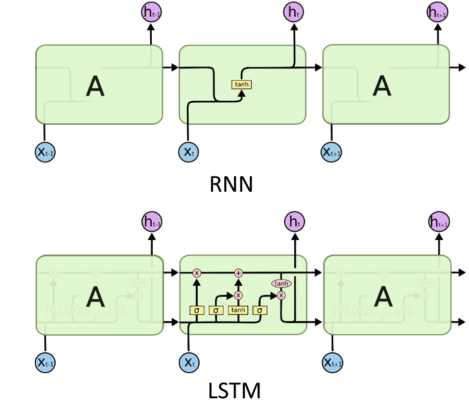
Image from https://colah.github.io/posts/2015-08-Understanding-LSTMs/
Before going on, in this representation the state unit is the horizontal line running through the top of the diagram.
Forget gate
The first thing we have to decide is if we want to keep the information in the cell state or if we want to throw it away. This is done by the forget gate, that for each number in the cell state will output a number between $0$ and $1$, by looking at $h_{t-1}$ and $x_t$.
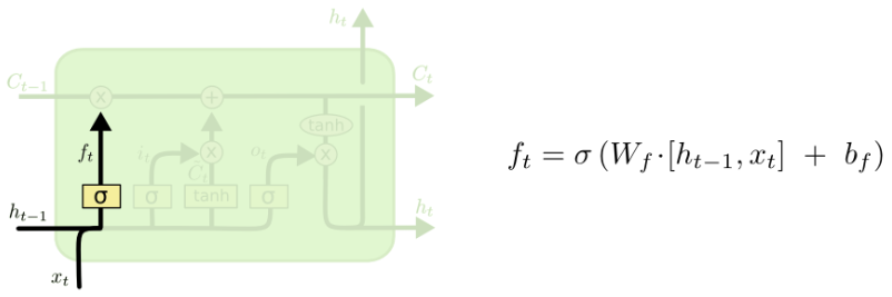
Image from https://colah.github.io/posts/2015-08-Understanding-LSTMs/
The input gate
Here we have two different operations: the input gate decides which values we will update, while a tanh layer creates a vector of new candidate values that could be added to the state.
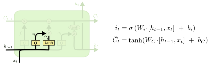
Image from https://colah.github.io/posts/2015-08-Understanding-LSTMs/
Update
In this step we only need to update the cell state by putting together the values coming from the forget gate and the input gate.
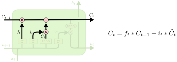
Image from https://colah.github.io/posts/2015-08-Understanding-LSTMs/
Output gate
In the last step, the output is computed by taking the cell state, putting it through a tanh and multiplying it by a sigmoid gate (notice that this sigmoid gate is essentially equal to the initial forget gate, but of course with its own parameters).
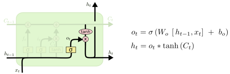
Image from https://colah.github.io/posts/2015-08-Understanding-LSTMs/
Look on the Christopher Olah’s blog post to see some variations of LSTMs, such as Gated Recurrent Unit (GRU), in which the main difference is that a single gating unit simultaneously controls the forgetting factor and the decision to update the state unit.