In this post we will talk about Linear Classification, explaining some of the main methods which are at the basis of this task.
Disclaimer: the following notes were written following the slides provided by the professor Restelli at Polytechnic of Milan and the book ‘Pattern Recognition and Machine Learning'.
Linear Classification
The goal in classification is to take an input vector $x$ and to assign it to one of $K$ discrete classes $C_k$ where $k = 1,…,K$. In the most common scenario these classes are disjoint, hence each input can belong to one and only one class. For this reason the input space is divided into the so called decision regions, whose boundaries are called decision boundaries or decision surfaces.
In this chapter we will talk about linear models for classification, so these decision surfaces are defined by $(D - 1)$-dimensional hyperplanes within the $D$-dimensional input space.
For regression problems, the target variable $t$ is simply the vector of real numbers whose values we wish to predict. In classification the representation can be different according to the context. For example, in the case of two-class problems, the most common choice is a single target variable $t \in {0,1}$, that can be interpreted as the probability of the class to be $C_1$ or $C_2$.
If instead we have more than two classes, we can expand the previous notation using a vector $\boldsymbol{t}$ where all elements are $0$ except from the one that represents the right class.
Another difference from the regression models is the model prediction. Indeed, instead of having $y(\boldsymbol{x},\boldsymbol{w}) = \boldsymbol{x}^T\boldsymbol{w} + w_0$, which as said is linear in the parameters, in linear classification models:
$$ y(\boldsymbol{x},\boldsymbol{w}) = f(\boldsymbol{x}^T\boldsymbol{w} + w_0) $$
where $f(\cdot)$ is a nonlinear function, called activation function.
Finally, to conclude this introduction, note that as for regression there can be used fixed nonlinear basis functions. In particular, the decision surfaces correspond to $y(\boldsymbol{x}) = constant$, hence they are linear functions of $x$. This is important because if the decision surface is linear, the input space must be linearly separable. If it is not the case, the main idea is to make a fixed nonlinear transformation of the input space, using a vector of basis functions $\phi(\boldsymbol{x})$.
Approaches to classification
-
Discriminant function (or direct approach): build a function the directly maps each input to a specific class.
-
Probabilistic approach
- Probabilistic discriminative approach: model $p(C_k|\boldsymbol{x})$ directly (e.g. logistic regression).
- Probabilistic generative approach: model $p(\boldsymbol{x}|C_k)$ and $p(C_k)$ and then using the Bayes’ rule:
$$ P(C_k|\boldsymbol{x}) = \frac{p(\boldsymbol{x}|C_k)p(C_k)}{p(\boldsymbol{x})} $$
Discriminant function (direct approach)
Two-class
Let’s consider a two-classes problem. Considering the following model
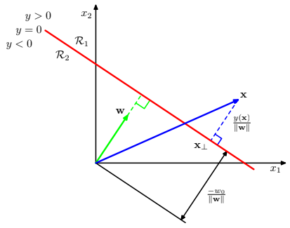
$$ y(\boldsymbol{x}) = \boldsymbol{x}^T\boldsymbol{w} + w_0 $$
a possible approach can be to assign $\boldsymbol{x}$ to $C_1$ if $y(\boldsymbol{x}) \geq 0$ and $C_2$ otherwise.
Let’s now consider two points that lie on the decision surface $x_A$ and $x_B$. Since they lie on the surface
$$ \displaylines{y(x_A) = y(x_B) = 0 \\ \boldsymbol{w}^T(x_A-x_B) = 0} $$
and this means that the vector $\boldsymbol{w}$ is orthogonal to every vector lying within the decision surface (scalar product = 0), and so $\boldsymbol{w}$ determines the orientation of the decision surface.
Let’s now consider a single point $x$ on the decision surface. As before, $y(x) = 0$, so
$$ \frac{\boldsymbol{w}^Tx}{||\boldsymbol{w}||} = -\frac{w_0}{||\boldsymbol{w}||} $$
hence the bias parameter $w_0$ determines the translation of the decision surface w.r.t. the origin.
Multiple classes
The first idea that can cross our mind is to put together a number of two-class discriminant functions. However, this can lead to some difficulties.
- ONE-VERSUS-THE-REST : $K-1$ classifiers each of which solves a two-class problem.
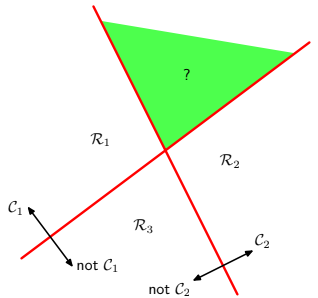
- ONE-VERSUS-ONE: $\frac{K(K-1)}{2}$ binary classifiers
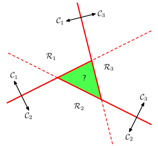
As we can see, both approaches lead to regions of input space that are ambiguously classified. The following approach solves this issue.
- Using $K$ linear discriminant functions of the form:
$$ y_k(x) = w_k^Tx + w_{k0} $$
and $x$ will be assigned to the class $C_k$ such that $y_k(x) > y_j(x) \ \forall j \ne k$
This means that the decision boundary between two generic classes $C_k$ and $C_j$ is the hyperplane identified by:
$$ y_k(x) = y_j(x) \implies (w_k-w_j)^Tx + (w_{k0}-w_{j0}) = 0 $$
This has the same form as the decision boundary for the two-class case, so analogous geometrical properties apply. However, this type of classifiers have the beautiful property of being simply connected and convex (it can be proved).
Least squares for classification
We know that for regression problems least squares can be a good choice, since it provides a simple closed-form solution. Can we apply it to classification? SPOILER: nope. Let’s see why.
Let’s consider a general classification problem with $K$ classes using 1-of-$K$ binary coding scheme for the target vector $\boldsymbol{t}$. This means that each class is described by its own linear model
$$ y_k(\boldsymbol{x}) = \boldsymbol{x}^T\boldsymbol{w_k} + w_{k0} $$
In a vector notation to group all the classes
$$ \boldsymbol{y}(\boldsymbol{x}) = \boldsymbol{\tilde{W}}^T\boldsymbol{\tilde{x}} $$
where $\tilde{W}$ is a $(D+1)$ x $K$ matrix, where each column is a weight vector of a different classifier.
The next step is to find the optimal weight matrix. Given a dataset $D = {x_i,t_i}$, where $i = 1,…,N$ and considering the loss function
$$ E_D(\boldsymbol{\tilde{W}}) = \frac{1}{2}Tr\{(\boldsymbol{\tilde{X}}\boldsymbol{\tilde{W}}-\boldsymbol{T})^T(\boldsymbol{\tilde{X}}\boldsymbol{\tilde{W}}-\boldsymbol{T})\} $$
where $Tr{}$ means the trace of the matrix. Minimizing least squares will lead to the already known closed-form solution
$$ \boldsymbol{\tilde{W}} = (\boldsymbol{\tilde{X}^T}\boldsymbol{\tilde{X}})^{-1}\boldsymbol{\tilde{X}^T\boldsymbol{T}} $$
What’s the problem?
Actually the problem is always the same: least squares is highly sensitive to outliers, as we can see from this image
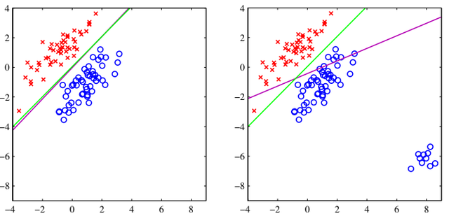
This is due to the loss function, that penalizes predictions which are “too correct” in that they lie a long way on the correct side of the decision boundary. However, this is not the only problem that affects least squares. Recall that it corresponds to maximum likelihood under the assumption of a Gaussian conditional distribution, but for sure binary target vectors have a distribution that is far from Gaussian.
Perceptron algorithm
Ok, let’s skip to another linear discriminant model: the perceptron of Rosenblatt (1962). Unlike least squares, which has a closed-form solution, it is an online linear classification algorithm. More precisely, it corresponds to a two-class model:
$$ y(\boldsymbol{x}) = f(\boldsymbol{w}^T\phi(\boldsymbol{x})) $$
where $f(\cdot)$ is a step function, i.e.
$$ \displaylines{f(a) = \begin{cases} +1 & {if } \ {a \geq 0} \\ -1 & {if } \ {a < 0} \end{cases}} $$
For sure to determine the parameters $\boldsymbol{w}$ we will try to minimize an error function. A natural choice of this error function would be the total number of misclassified patterns. However, doing so the error will be a piecewise constant function of $\boldsymbol{w}$, with discontinuities wherever a change in $\boldsymbol{w}$ causes the decision boundary to move across one of the data points. For this reason we cannot use methods based on the gradient, because the latter is zero almost everywhere.
That’s why there is a specific error function, called perceptron criterion:
$$ L_P(\boldsymbol{x}) = -\sum_{n \in \mathcal{M}}\boldsymbol{w}^T\phi_n(\boldsymbol{x_n})t_n $$
where $\mathcal{M}$ is the set of misclassified points.
The idea is that the algorithm finds the separating hyperplane by minimizing the distance of misclassified points to the decision boundary. The contribution to the error associated with a particular misclassified pattern is a linear function of $\boldsymbol{w}$ in regions of $\boldsymbol{w}$ where the pattern is misclassified and zero in regions where it is correctly classified. The total error function is therefore piecewise linear. Note that the minus in the loss function is a trick to make it always positive, since in the summation $\boldsymbol{w}^T\phi_n(x_n)t_n$ is always negative (remember that we are considering only misclassified points).
So, how do we minimize this loss function? Stochastic gradient descent.
$$ \boldsymbol{w}^{(k+1)} = \boldsymbol{w}^k - \eta\nabla L_P(\boldsymbol{w}) = \boldsymbol{w}^{(k)} + \eta\phi(\boldsymbol{x_n})t_n $$
where $\eta$ is the learning rate and $k$ represents the steps of the algorithm. Since if we multiply $\boldsymbol{w}$ by a constant the perceptron function is unchanged, we can set $\eta = 1$.
In a nutshell, the algorithm does the following: we cycle through the training patterns and for each of them we evaluate the perceptron function. If the pattern is correctly classified, then the weight vectors remains unchanged, otherwise for class $C_1$ we add the vector $\phi(\boldsymbol{x_n})$ to the current estimate of $\boldsymbol{w}$, while for class $C_2$ we subtract it from $\boldsymbol{w}$.
Some observation:
- the perceptron learning rule is not guaranteed to reduce the total error function at each stage.
- the perceptron convergence theorem states that if the input space is linearly separable, then the perceptron algorithm is guaranteed to find an exact solution in a finite number of steps. However, note that the number of steps could be substantial and in practice, until convergence is achieved, we will not be able to distinguish between a nonseparable problem and one that is simply slow to converge!
In addition to the difficulties with the learning algorithm, the perceptron does not provide probabilistic outputs, does not generalize to $K>2$ classes and, as all the models we’ve seen, it is based on linear combinations of fixed basis functions.
That is why we are going to skip to a more powerful model.
Probabilistic Discriminative Models
Logistic Regression
First of all, note that even if the name can be tricky, logistic regression is a CLASSIFICATION algorithm.
Logistic regression can be seen as a special case of the generalized linear model and thus analogous to linear regression. The model of logistic regression, however, is based on quite different assumptions (about the relationship between dependent and independent variables) from those of linear regression. In particular the key differences between these two models can be seen in the following two features of logistic regression:
- First, the conditional distribution $y \mid x$ is a Bernoulli distribution rather than a Gaussian distribution, because the dependent variable is binary.
- Second, the predicted values are probabilities and are therefore restricted to (0,1) through the logistic distribution function because logistic regression predicts the probability of particular outcomes rather than the outcomes themselves.
Without entering too much in the details, under rather general assumptions, the posterior probability of class $C_1$ can be written as a logistic sigmoid acting on a linear function of the feature vector $\phi$, so that
$$ p(C_1|\phi) = \frac{1}{1+e^{-\boldsymbol{w}^T\phi}} = \sigma(\boldsymbol{w}^T\phi) $$
with $p(C_2|\phi) = 1 - p(C_1|\phi)$
An important advantage of logistic regression is that for an $M$-dimensional feature space $\phi$, it has $M$ adjustable parameters, while if we had fitted Gaussian class conditional densities using maximum likelihood we would have used $\sim M^2$ parameters.
We now used maximum likelihood to determine the parameters of the logistic regression models. To do this, note this beautiful property:
$$ \frac{d\sigma}{da} = \sigma(1-\sigma) $$
So, given a dataset $D =$ {$\phi_n,t_n$}, $t_n \in$ {$0,1$}, applying ML means maximizing the probability of getting the right label:
$$ p(\boldsymbol{t}|\boldsymbol{X},\boldsymbol{w}) = \prod_{n=1}^{N}y_n^{t_n}(1-y_n)^{1-t_n}, \ y_n = \sigma(\boldsymbol{w}^T\phi_n) $$
As usual, we can define an error function by taking the negative logarithm of the likelihood, which gives the cross-entropy error function:
$$ L(\boldsymbol{w}) = -ln \ p(\boldsymbol{t}|\boldsymbol{X},\boldsymbol{w}) = -\sum_{n=1}^{N}(t_n \ ln \ y_n + (1-t_n) \ ln \ (1-y_n)) = \sum_{n=1}^{N}L_n $$
Taking the gradient of the error function with respect to $\boldsymbol{w}$, we obtain
$$ \frac{\partial L_n}{\partial y_n} = \frac{y_n-t_n}{y_n(1-t_n)} $$
$$ \frac{\partial y_n}{\partial \boldsymbol{w}} = y_n(1-y_n)\phi_n $$
$$ \frac{\partial L_n}{\partial \boldsymbol{w}} = \frac{\partial L_n}{\partial y_n}\frac{\partial y_n}{\partial \boldsymbol{w}} = (y_n-t_n)\phi_n $$
$$ \implies \nabla L(\boldsymbol{w}) = \sum_{n=1}^{N}(y_n-t_n)\phi_n $$
Note that it takes precisely the same form as the gradient of the sum-of-squares error function for the linear regression model, but in this case $y$ is not a linear function of $\boldsymbol{w}$, so there is no closed-form solution. However, the error function is convex, hence it can be optimized by standard gradient-based optimization techniques (can be adapted also to the online learning setting).
Multiclass Logistic Regression
For the multiclass case, the posterior probabilities can be represented by a softmax transformation of linear functions of the feauture variables, so that
$$ p(C_k|\phi) = y_k(\phi) = \frac{e^{\boldsymbol{w_k}^T\phi}}{\sum_{j}e^{\boldsymbol{w_j}^T\phi}} $$
In mathematics, the softmax function, also known as softargmax or normalized exponential function, is a function that takes as input a vector of $K$ real numbers, and normalizes it into a probability distribution consisting of $K$ probabilities. That is, prior to applying softmax, some vector components could be negative, or greater than one, and might not sum to 1; but after applying softmax, each component will be in the interval $(0,1)$, and the components will add up to $1$, so that they can be interpreted as probabilities. Furthermore, the larger input components will correspond to larger probabilities.
As before, we use ML to determine directly the parameters
$$ p(\boldsymbol{T}|\Phi,\boldsymbol{w_1},…,\boldsymbol{w_K}) = \prod_{n=1}^{N}(\prod_{k=1}^{K}p(C_k|\phi_n)^{t_{nk}}) = \prod_{n=1}^{N}(\prod_{k=1}^{K}y_{nk}^{t_{nk}}) $$
where $y_{nk} = p(C_k|\phi_n)$
The cross-entropy function is
$$ L(\boldsymbol{w_1},…,\boldsymbol{w_K}) = -ln \ p(\boldsymbol{T}|\Phi,\boldsymbol{w_1},…,\boldsymbol{w_K}) = -\sum_{n=1}^{N}(\sum_{k=1}^{K}t_{nk}ln \ y_{nk}) $$
Taking the gradient
$$ \nabla L_{\boldsymbol{w_j}}(\boldsymbol{w_1},…,\boldsymbol{w_K}) = \sum_{n=1}^{N}(y_{nj}-t_{nj})\phi_n $$
Probabilistic Generative Models
Generative models have the purpose of modeling the joint probability density function of the couple input/output $p(C_k,\boldsymbol{x})$, which allows to generate also new data from what has been learned.
Naive Bayes
There is not a single algorithm for training this type of classifiers, but a family of algorithms based on a common principle: the assumption that each input is conditionally (w.r.t the class) independent from each other.
$$ \displaylines{p(C_k|\boldsymbol{x}) = \frac{p(C_k)p(\boldsymbol{x}|C_k)}{p(\boldsymbol{x})} \propto p(x_1,…,x_M,C_k) \\ = p(x_1|x_2,…,x_M,C_k)p(x_2,…,x_M,C_k) \\ = p(x_1|x_2,…,x_M,C_k)p(x_2|x_3,…,x_M,C_k)p(x_3,…,x_M,C_k) \\ = p(x_1|x_2,…,x_M,C_k)p(x_2|x_3,…,x_M,C_k)…p(x_{M-1}|x_M,C_k)p(x_M|C_k)p(C_k) \\ = p(C_k)\prod_{j=1}^{M}p(x_j|C_k)} $$
The decision function, that maximizes the MAP probability, is the following:
$$ y(\boldsymbol{x}) = arg \ max_k \ p(C_k) \prod_{j=1}^{M}p(x_j|C_k) $$
A class’s prior may be calculated by assuming equiprobable classes, i.e. $p(C_k) = \frac{1}{K}$. The assumptions on distributions of features are called the event model of the Naive Bayes classifier. For discrete features, multinomial and Bernoulli distributions are popular.
When dealing with continuous data, a typical assumption is that the continuous values associated with each class are distributed according to a Gaussian distribution. For example, suppose the training data contains a continuous attribute, $x$. We first segment the data by the class, and then compute the mean and variance of $x$ in each class.
Let $\mu_k$ be the mean of the values in $x$ associated with class $C_k$, and let $\sigma_k^2$ be the variance of the values in $x$ associated with class $C_k$. Suppose we have collected some observation value $v$. Then, the probability distribution of $v$ given a class $C_k$, $p(x=v|C_k)$, can be computed by plugging $v$ into the equation for a Normal distribution parameterized by $\mu_k$ and $\sigma_k^2$. That is,
$$ p(x=v|C_k) = \frac{1}{\sqrt{2\pi\sigma_k^2}}e^{-\frac{(v-\mu_k)^2}{2\sigma_k^2}} $$
Non-parametric methods
Algorithms that do not make strong assumptions about the form of the mapping function are called nonparametric machine learning algorithms. By not making assumptions, they are free to learn any functional form from the training data.
“Nonparametric methods are good when you have a lot of data and no prior knowledge, and when you don’t want to worry too much about choosing just the right features.” Artificial Intelligence: A Modern Approach
K-nearest neighbor
k-NN is a type of instance-based learning, or lazy learning, where the function is only approximated locally and all computation is deferred until classification. Note indeed that the training phase is practically absent, but the prediction phase is quite slow, since it must iterate over all the data points every time.
For each sample to predict, the closest k samples are selected and the label belonging to the majority of them is assigned to the new sample. If k is even, a policy for breaking the ties has to be chosen, e.g. randomly.
The concept of closest requires the definition of a similarity measure, which is not always trivial but that has the advantage of the possibility to use K-NN also for objects (such as graphs) for which a similarity can be defined.
It is affected by the curse of dimensionality, which means that having a very high number of dimensions will decrease the performance of the predictor. The curse is caused by the fact that with high dimensions, all the points tend to have the same distance from one to another.
The choice of the k parameter is very important for the performance of the algorithm and it can be chosen through cross-validation. A very low k will have high variance and low bias, while a high k will have a low variance but high bias.
Performance measures
We are at the end! To conclude this chapter we’re going to answer the question: how can we evaluate the performance of a method?
Confusion matrix
The confusion matrix is a simple table which shows the number of points that have been correctly classified and those that have been misclassified.
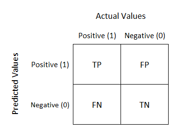
From this matrix we can compute the following useful metrics:
- Accuracy: $\frac{tp+tn}{N}$, fraction of the samples correctly classified in the dataset
- Precision: $\frac{tp}{tp+fp}$, fraction of samples correctly classified in the positive class among the ones classified in the positive class
- Recall: $\frac{tp}{tp+fn}$, fraction of samples correctly classified in the positive class among the ones belonging to the positive class