In this post we will analyze Linear Regression Models in a pretty much detailed way, discussing the different approaches in which the problem can be tackled and also explaining what is regularization.
Disclaimer: the following notes were written following the slides provided by the professor Restelli at Polytechnic of Milan and the book ‘Pattern Recognition and Machine Learning'.
The goal of regression is to predict the value of one or more continuous target variables $t$ given the value of a D-dimensional vector $\boldsymbol{x}$ of input variables.
Linear models are simple and ofter provide an adequate and interpretable description of how the inputs affect the output. They can sometimes outperform fancier nonlinear models, especially in situations with small numbers of training cases, low signal-to-noise or sparse data.
The simplest form of linear regression models are also linear functions of the input variables:
$$ y(x,w) = w_0 + \sum_{j=1}^{D-1}w_jx_j $$
where the $w_j$'s are unknows parameters or coefficients and the variables ${x_j}$ can come from different sources.
However, this formulation imposes significant limitations on the model. That is why we can generalize a bit introducing the so called basis functions, i.e. linear combinations of fixed nonlinear functions of the input variables:
$$ y(x,w) = w_0 + \sum_{j=1}^{M-1}w_j\phi_j(x) $$
Using nonlinar basis functions, we allow the function $y(x,w)$ to be a nonlinear function of the input vector $\boldsymbol{x}$. It is important to underline that still the model is linear in $\boldsymbol{w}$, which brings some simplifications.
Some examples of basis functions are the following:
-
Polynomial $\rightarrow \phi_j(x) = x^j$
-
Gaussian $\rightarrow \phi_j(x) = e^{-\frac{(x-\mu_j)^2}{2\sigma^2}}$
-
Sigmoidal $\rightarrow \phi_j(x) = \frac{1}{1+e^{(\mu_j-x)/\sigma}}$
How can we estimate $\boldsymbol{w}$?
Typically what we have is a set of training data $(x_1, y_1)…(x_N,y_N)$ from which we estimate the parameters $\boldsymbol{w}$.
A common choice to do this estimation is least squares, with which we minimize the residual sum of squares:
$$ RSS(\boldsymbol{w}) = \sum_{n=1}^{N}(y(x_n, \boldsymbol{w}) - t_n)^2 $$
Actually, for convenience, the loss function is usually described as:
$$ E(\boldsymbol{w}) = \frac{1}{2}RSS(\boldsymbol{w}) = \frac{1}{2}\sum_{n=1}^{N}(y(x_n, \boldsymbol{w}) - t_n)^2 $$
Observation: it is a nonnegative quantity, that can be zero only if the function $y(x,\boldsymbol{w})$ passes exactly through each data point.

Now that we have our loss function we have to minimize it, hence choose $\boldsymbol{w}$ so that $E(\boldsymbol{w})$ is as small as possible. Since the error function is a quadratic function of the coefficients $\boldsymbol{w}$, its derivative with respect to them will be linear, and so the minimization has a unique solution, denoted by $\boldsymbol{w^*}$.
Let’s start by saying that the residual sum of squares $RSS$ can be also written as the sum of the $l_2$-norm of the vector of the residual errors:
$$ RSS(\boldsymbol{w}) = ||\epsilon||_2^2 = \sum^{N}\epsilon_i^2 = \epsilon^T\epsilon $$
This formulation simplifies the way in which we will write $RSS$ in its matrix form.
Let $\Phi = (\phi(x_1), \phi(x_2), …, \phi(x_N))^T$ and $t = (t_1, …, t_N)^T$.
$\epsilon = \boldsymbol{t}-\Phi\boldsymbol{w}$
So, from the previous $RSS$ formula, we can write:
$$ L(\boldsymbol{w}) = \frac{1}{2}RSS(\boldsymbol{w}) = \frac{1}{2}(\boldsymbol{t}-\Phi\boldsymbol{w})^T(\boldsymbol{t}-\Phi\boldsymbol{w}) $$
Finally, we can obtain the minimum imposing the gradient to be zero and the curvature to have all the eigenvalues > 0.
- First derivative
$$ \frac{\partial L(\boldsymbol{w})}{\partial \boldsymbol{w}} = -\Phi^T(\boldsymbol{t}-\Phi\boldsymbol{w}) $$
- Second derivative
$$ \frac{\partial^2 L(\boldsymbol{w})}{\partial \boldsymbol{w} \partial \boldsymbol{w}^T} = \Phi^T\Phi $$
If we assume that $\Phi^T\Phi$ is nonsingular (hence invertible), it is symmetric and positive semi-definite, so all the eigenvalues are $\geq 0$.
Setting the gradient to zero gives
$$ \displaylines{-\Phi^T(\boldsymbol{t}-\Phi\boldsymbol{w}) = 0 \\ \Phi^T\Phi\boldsymbol{w} = \Phi^Tt \\ \boldsymbol{w}_{OLS} = (\Phi^T\Phi)^{-1}\Phi^Tt} $$
Discriminative approach
What we have seen so far is called a direct approach, i.e. find a regression function directly from the training data by searching in the space of the model (changing the parameters). Now we will introduce a discriminative approach, where we model directly the conditional density $p(t|x)$.
Let’s assume that the target variable $t$ is given by a deterministic function $y(x,w)$ with additive Gaussian noise:
$$ t = y(x,w) + \epsilon $$
where $\epsilon \sim \mathcal{N}(0,\sigma^2)$
Hence $t \sim \mathcal{N}(y(x,w),\sigma^2)$
Now consider a data set of inputs $$X = {x_1, …, x_N}$$ with corresponding target values $t_1, …, t_N$. Under the assumption that these data points are independent and identically distributed (i.i.d.), the likelihood function is:
$$ p(\boldsymbol{t}|\boldsymbol{X},\boldsymbol{w},\sigma^2) = \prod_{n=1}^{N}\mathcal{N}(t_n|\boldsymbol{w}^T\phi(x_n), \sigma^2) = \prod_{n=1}^{N}\frac{1}{2\pi\sigma^2}e^{-\frac{(t-y(x,w))^2}{2\sigma^2}} $$
Recall that if we assume a squared loss function then the optimal prediction for a new value of $x$ will be given by the conditional mean of the target variable. That is why now we need to use $\boldsymbol{w}$ to approximate the mean of the Gaussian.
This can be done by finding the maximum likelihood:
$$ \displaylines{l(\boldsymbol{w}) = ln \ p(\boldsymbol{t}|\boldsymbol{X},\boldsymbol{w},\sigma^2) = \sum_{n=1}^{N}ln \ p(t_n|x_n,\boldsymbol{w},\sigma^2) \\ = -\frac{N}{2}ln(2\pi\sigma^2) - \frac{1}{2\sigma^2}RSS(\boldsymbol{w}) \\ = -\frac{N}{2}ln(2\pi\sigma^2)-\frac{1}{4\sigma^2}(\boldsymbol{t}-\boldsymbol{w}\Phi)^T(\boldsymbol{t}-\boldsymbol{w}\Phi)} $$
Now we compute the gradient:
$$ \displaylines{\nabla ln \ l(\boldsymbol{W}) = -\Phi^T(\boldsymbol{t}-\Phi\boldsymbol{w}) = -\Phi^T\boldsymbol{t}+\Phi^T\Phi\boldsymbol{w} = 0 \\ \boldsymbol{w_{ML}} = (\Phi^T\Phi)^{-1}\Phi^T\boldsymbol{t}} $$
which are known as the normal equations for the least squares problem. Here $\Phi$ is a $NxM$ matrix, called the design matrix.
The quantity $(\Phi^T\Phi)^{-1}\Phi^T$ is known as the Moore-Penrose pseudo-inverse of the matrix $\Phi$. It can be seen as a generalization of the matrix inversion operation, since it applies also to nonsquare matrices.
What happens when $\Phi^T\Phi$ is close to singular?
Well, in that case a direct solution of the normal equations can lead to numerical difficulties, i.e. the resulting parameter values can have large magnitudes. Unfortunately, when dealing with real dataset, this situation often happens. One way to solve this issue is using the so called singular value decomposition.
Another way (very common), is the regularization, which prevents this issue to happen, ensuring that the matrix is nonsingular.
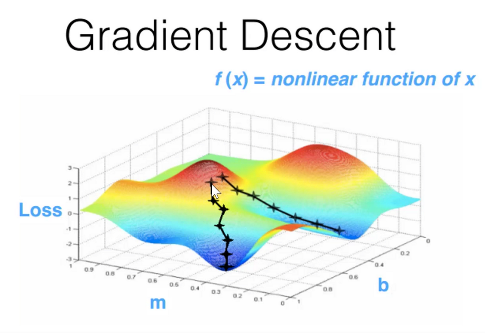
Learning with stochastic gradient descent (SGD)
Ok, at this point one could think that the technique we’ve seen so far is computationally expensive. And that is true. Indeed, we are processing the entire training set in one go, and this can be very costly if we’re dealing with a very large dataset.
So, in this case a good idea could be using an online algorithm, in which the gradient is computed one sample at a time.
The most famous and used algorithm is the stochastic gradient descent.
This algorithm updates the parameter vector $\boldsymbol{w}$ in the following way:
$$ \boldsymbol{w}^{k+1} = \boldsymbol{w}^k - \eta\nabla E_n $$
where $k$ indicates the iteration number and $\eta$ the learning rate. Choosing the right $\eta$ is not an easy task, since if the value is too high or too low, it could prevent the algorithm to converge.
Regularization
Before talking about regularization it is worth to underline two concepts: underfitting and overfitting.
As we said before, linear models can be generalized using the basis functions, which increase the complexity of our model trying to overcome the limitations imposed by the simplest form of linear regression.
The problem lies in this “complexity”: how complex should our model be in order to fit the data in the best way? As often we have to find a tradeoff.
- A model with low complexity is usually not capable of fitting the data and so representing appropriately the true model, underfitting.
- A model with high complexity, instead, may fit very well the training data, but does not generalize on unseen data, overfitting.
As we will see there are techniques to overcome these issues, expecially overfitting. However we’ll have to deal with another tradeoff between variance and bias. One thing that reduces overfitting without any drawback is increasing the size of our dataset, but of course this is not always possible.
Regularization consists of adding a penalty term to the loss function to discourage the coefficients from reaching large values.
Ridge regression
$$ L(\boldsymbol{w}) = \frac{1}{2}\sum_{n=1}^{N}{(t_n - \boldsymbol{w}^T\phi(x_n))^2} \ + \ \frac{\lambda}{2}\boldsymbol{w}^T\boldsymbol{w} $$
This particular choice of regularizer is known as ridge regression or weight decay, since in online learning algorithms it encourages weigth values to decay towards zero, unless supported by the data.
The advantage of Ridge regression is that the loss function remains quadratic in $\boldsymbol{w}$, so its exact minimizer can be found in closed form.
Lasso regression
$$ L(\boldsymbol{w}) = \frac{1}{2}\sum_{n=1}^{N}{(t_n - \boldsymbol{w}^T\phi(x_n))^2} \ + \ \frac{\lambda}{2}||\boldsymbol{w}||_1 $$
In this case no closed-form solution exists, however if $\lambda$ is sufficiently large, some of the coefficients $w_j$ are driven to zero, leading to a sparse model.
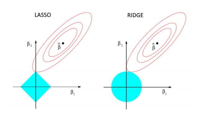
In the picture above we can see where the origin of sparsity in Lasso comes from: the optimum value $\boldsymbol{w}^*$ will probably be on one of the vertices, hence on the axes, where some features are zero (the features in the image are indicated as $\beta_j$). $\$ In cases of multi-correlation, i.e. many features are correlated with each other, this can be useful as the Lasso regression will set some of them to zero and leave the others to do their job.
Bayesian Linear Regression
Till now we have adopted a frequentist approach, namely we’ve seen the probabilities in terms of frequencies of random, repeatable events. Sometimes, however, it’s not possible to repeat multiple times an event to obtain a notion of probability. Moreover, we’ve also seen that using maximum likelihood for setting the parameters we have the problem of the model complexity. Regularization is a good answer, but still, the choice of the basis functions remains important and also the value of $\lambda$ is an incognita.
Here the Bayesian approach comes into play. This approach can be splitted in the following steps:
- We enumerate all the reasonable models of the data and we assign a prior distribution $p(\boldsymbol{w})$ to each of these models.
- We observe the data and we evaluate how probable the data was under each of these models, computing $p(D|\boldsymbol{w})$.
- From the previous observation we compute a posterior distribution $p(\boldsymbol{w}|D)$, which encapsulates everything that you have learned from the data regarding the possible models under consideration.
An important consideration is that this approach is not affected by the problem of overfitting and it also leads to automatic methods of determining model complexity using the training data alone.
Posterior distribution
$$ p(\boldsymbol{w}|D) = \frac{p(D|\boldsymbol{w})p(\boldsymbol{w})}{P(D)} $$
where $P(D)$ is a normalizing constant.
In other words, the above formula means that
$$ posterior \propto likelihood \cdot prior $$
Here we can observe the two primary benefits of Bayesian Linear Regression:
- Priors: If we have domain knowledge, or a guess for what the model parameters should be, we can include them in our model, unlike in the frequentist approach which assumes everything there is to know about the parameters comes from the data. If we don’t have any estimates ahead of time, we can use non-informative priors for the parameters such as a normal distribution.
- Posterior: The result of performing Bayesian Linear Regression is a distribution of possible model parameters based on the data and the prior. This allows us to quantify our uncertainty about the model: if we have fewer data points, the posterior distribution will be more spread out.
The formulation of model parameters as distributions encapsulates the Bayesian worldview: we start out with an initial estimate, our prior, and as we gather more evidence, our model becomes less wrong. Bayesian reasoning is a natural extension of our intuition. Often, we have an initial hypothesis, and as we collect data that either supports or disproves our ideas, we change our model of the world.
Another important property of the Bayesian approach is that when new data are available, it is possible to use the posterior value as prior to compute the new posterior. This is true under the assumption of i.i.d. data and that the prior and posterior have the same distribution. This latter fact introduces the concept of conjugate priors:
for a given probability distribution, we can seek a prior that is conjugate to the likelihood function, so that the posterior has the same distribution as the prior. For example the prior of a Gaussian is a Gaussian and the prior of a Beta is a Bernoulli.
Back to math
As said, in the Bayesian approach the parameters are considered as drawn from some distribution. Assuming a Gaussian likelihood model, the conjugate prior is Gaussian too:
$$ p(\boldsymbol{w}) = \mathcal{N}(\boldsymbol{w}|\boldsymbol{w_0},\boldsymbol{S_0}) $$
Given the data $D$, we compute the posterior distribution, which is proportional to the product of the likelihood function and the prior and that is still a Gaussian:
$$ p(\boldsymbol{w}|\boldsymbol{t},\Phi,\sigma^2) \propto \mathcal{N}(\boldsymbol{w}|\boldsymbol{w_0},\boldsymbol{S_0})\mathcal{N}(\boldsymbol{t}|\Phi\boldsymbol{w},\sigma^2\boldsymbol{I_N}) = \mathcal{N}(\boldsymbol{w}|\boldsymbol{w_N},\boldsymbol{S_N}) $$
where
$$ \displaylines{\boldsymbol{w_N} = \boldsymbol{S_N}(\boldsymbol{S_0}^{-1}\boldsymbol{w_0}+\frac{\Phi^T\boldsymbol{t}}{\sigma^2}) \\ \boldsymbol{S_N}^{-1} = \boldsymbol{S_0}^{-1} + \frac{\Phi^T\Phi}{\sigma^2}} $$
Since the posterior distribution is Gaussian, its mode coincides with its mean, so $\boldsymbol{w_N}$ is the MAP estimator. Notice that in many cases we may have little idea of what form the distribution should take. We may then seek a form or prior distribution, called a noninformative prior, which is intended to have as little influence on the posterior distribution as possible. This is sometimes referred to as “letting the data speak for themselves”.
In such cases, the value of $\boldsymbol{S_0} \rightarrow \infty$, so
$$ \boldsymbol{S_N}^{-1} \rightarrow 0 \ + \frac{\Phi^T\Phi}{\sigma^2} \Rightarrow \boldsymbol{S_N} = \sigma^2(\Phi^T\Phi)^{-1} \Rightarrow \boldsymbol{w_N} = \sigma^2(\Phi^T\Phi)^{-1}\frac{\Phi^T\boldsymbol{t}}{\sigma^2} = (\Phi^T\Phi)^{-1}\Phi^T\boldsymbol{t} $$
which is the ordinary least squares solution! So, $\boldsymbol{w_N}$ reduces to the ML estimator. If $\boldsymbol{w_0} = 0$ and $\boldsymbol{S_0} = \tau^2\boldsymbol{I}$, then ${\boldsymbol{w_N}}$ reduces to the ridge estimate, where $\lambda = \frac{\sigma^2}{\tau^2}$
Indeed, doing ridge regression means doing bayesian linear regression when you put Gaussian prior centered in zero. Changing $\lambda$ means changing $\tau^2$, i.e. the variance of the prior.
Predictive distribution
Said this, in practice, we are not usually interested in the value of $\boldsymbol{w}$ itself, but rather in making predictions of t for new values of x. This requires that we evaluate the predictive distribution defined by:
$$ \displaylines{p(t|x,D,\sigma^2) = \int\mathcal{N}(t|\boldsymbol{w}^T\phi(x),\sigma^2)\mathcal{N}(\boldsymbol{w}|\boldsymbol{w_N},\boldsymbol{S_N})d\boldsymbol{w} = \mathcal{N}(t|\boldsymbol{w_N}^T\phi(x),\sigma_N^2(x)) \\ \sigma_N^2(x) = \sigma^2 + \phi(x)^T\boldsymbol{S_N}\phi(x)} $$
where $\sigma^2$ represents the noise in the target values (irreducible noise) and $\phi(x)^T\boldsymbol{S_N}\phi(x)$ the uncertainty associated with parameter values. As additional data points are observed, the second term becomes smaller and smaller. We can see this from this image:
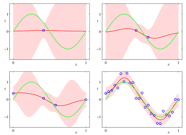
The green curve represents the function $sin(2\pi x)$, from which the data points are generated (with the addition of Gaussian noise). The red curve shows the mean of the corresponding Gaussian predictive distribution, while the pink region spans one standard deviation either side of the mean, and as we can see it never goes to zero, because of the intrinsic noise in the samples.