In this post I will introduce the Object Localization and Detection task, starting from the most straightforward solutions, to the best models that reached state-of-the-art performances, i.e. R-CNN, Fast R-CNN, Faster R-CNN and YOLO.
Disclaimer: These notes are for the most part a collection of concepts taken from the slides of the ‘Artificial Neural Networks and Deep Learning’ course at Polytechnic of Milan and from some other online resources. I am just putting together all the information to study for the exam and I thought it would be a good idea to upload them here since they can be useful for someone interested in this topic.
Object Localization and Detection
Localization
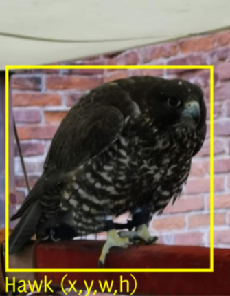
In localization, the input image contains a single relevant object to be classified in a fixed set of categories.
The task is:
- assign the object class to the image
- locate the object in the image by its bounding box
The simplest solution
The most straightforward idea can be the following: since we need to predict both the class label and the bounding box, we can train a network to predict both. That is usually done by attaching another fully connected layer on the last convolution layer.
By doing this, we need to use a specific loss function, more precisely a multitask loss, which combines two different losses, one for the class label predictions (classification) and the other for the bounding box predictions (regression):
$$ L(x) = \alpha S(x) + (1 - \alpha) R(x) $$
where $\alpha$ is a hyperparameter of the network.
Note that this approach works only for one object at a time.
Weakly-Supervised Localization
As far as we have seen until now, our training dataset must be composed of annotated images with labels and a bounding box for each object. In order to avoid this expensive representation, weakly-supervised localization can be used.
The idea is to perform localization by getting rid of the annotated bounding boxes.
The Global Average Pooling revisited
Reference paper: Learning Deep Features for Discriminative Localization
While this technique was previously proposed as a means for regularizing training, we find that it actually builds a generic localizable deep representation that exposes the implicit attention of CNNs on an image. Despite the apparent simplicity of global average pooling, we are able to achieve 37.1% top-5 error for object localization on ILSVRC 2014 without training on any bounding box annotation.
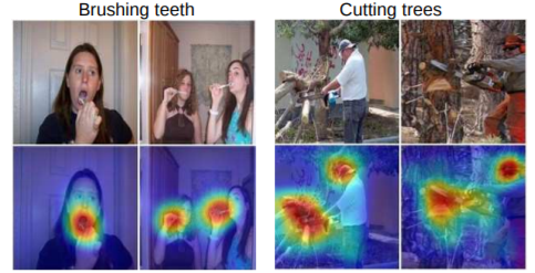
Image from Learning Deep Features for Discriminative Localization
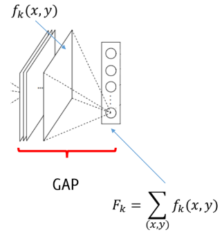
How can we obtain such results? If we consider a standard architecture made only of convolutions and activation functions, we know that it leads to a final layer having $n$ feature maps $f_k(:,:)$ having resolution “similar” to the input image. At this point global average pooling is performed, giving a vector made of $n$ averages $F_k$.
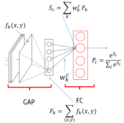
We then add and train a fully connected layer after the GAP. This FC computes $S_c$ for each class $c$ by the weighted sum of ${F_k}$, where weights are defined during training. Finally, the class probability $P_c$ is computed via softmax.
$$ S_c = \sum_{k} w_k^c F_k $$
where $w_k^c$ represents the importance of $F_k$ for the class $c$.
However, we can also write
$$ S_c = \sum_{k} w_k^c \sum_{x,y} f_k(x,y) = \sum_{x,y}\sum_{k} w_k^c f_k(x,y) $$
and $M_c(x,y) = \sum_{k} w_k^c f_k(x,y)$ is exactly the so-called **Class Activation Mapping (CAM)**, indicating the importance of the activations at $(x,y)$ for predicting the class $c$.
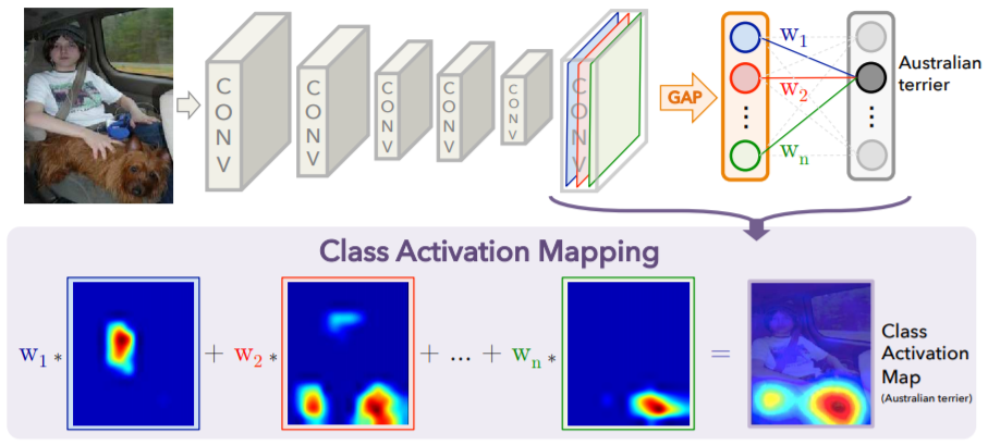
Image from Learning Deep Features for Discriminative Localization
As written in the paper, weakly supervised object localization was already tried by Oquab et al with Global Max Pooling. The idea behind the use of GAP is that it encourages the network to identify the extent of the object as compared to GMP which encourages it to identify just one discriminative part.
Object Detection
Task: given a fixed set of categories and an input image which contains an unknown and varying number of instances, draw a bounding box on each object instance.
The sliding window approach
The sliding window approach is the most straightforward solution. We simply apply a standard CNN to each crop of the image, sliding on it a window of fixed size and classifying each region.
The problems of this solution are clear:
- very inefficient, since it doesn’t use features that are “shared” among overlapping crops
- how can we choose the crop size?
- difficult to detect objects at different scales
- a huge number of crops of different sizes should be considered
The only advantage is that there is no need to retrain the CNN.
Region proposals
Region proposal algorithms (and networks) are meant to identify bounding boxes that correspond to a candidate object in the image. Thus, RCNN (Regions + CNN) consists of applying a region proposal algorithm and classify the image inside each proposal region by using a CNN.
R-CNN
Reference paper: Rich feature hierarchies for accurate object detection and semantic segmentation
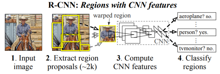
Image from Rich feature hierarchies for accurate object detection and semantic segmentation
Our approach combines two key insights: (1) one can apply high-capacity convolutional neural networks (CNNs) to bottom-up region proposals in order to localize and segment objects and (2) when labeled training data is scarce, supervised pre-training for an auxiliary task, followed by domain-specific fine-tuning, yields a significant performance boost.
Considering the above image, the Extract region proposal step can be performed with many different techniques, since, as said in the paper, R-CNN is agnostic to the particular region proposal method. Then, there is the Feature extraction phase, in which a standard CNN is used. Note that before this, the extracted regions are warped to a predefined size in order to make them compatible with the CNN (because of the FC layer at the end). In the last step, SVM + BB regressor are used to classify regions. A linear SVM per class is used to classify between object and background (an IoU overlap threshold is used to deal with cases in which the object and the background overlap), while the Bounding Box regressor is used to improve localization performance, by refining the region proposals using the features computed by the CNN.
The CNN of the paper was discriminatively pretrained on a large auxiliary dataset and then fine-tuned to adapt it to the new task and the new domain.
Limitations
- Ad-hoc training objectives and not an end-to-end training
- Fine-tune network with softmax classifier (log loss)
- Train post-hoc linear SVMs (hinge loss)
- Train post-hoc bounding box regressions (least squares)
- Region proposals are from a different algorithm, thus that part has not been optimized for the detection by CNN
- Training is slow and takes a lot of space to store features
- Also inference is slow, since the CNN has to be executed on each region proposal (no feature re-use)
Fast R-CNN
Reference paper: Fast R-CNN
Compared to previous work, Fast R-CNN employs several innovations to improve training and testing speed while also increasing detection accuracy.
R-CNN is slow because it performs a ConvNet forward pass for each object proposal, without sharing computation.
Advantages of Fast R-CNN:
- Higher detection quality (mAP) than R-CNN and SPPnet (the latter is another architecture, which solves some problems of R-CNN)
- Training is single-stage, using a multi-task loss
- Training can update all network layers
- No disk storage is required for feature caching
Fast R-CNN takes as input an entire image and a set of object proposals. The network first processes the image with several convolutional and max pooling layers, and then, for each object proposal, a region of interest (RoI) pooling layer, followed by fully connected layers, extracts a fixed-length feature vector from the feature map. Then, the network has two output vectors per RoI: softmax probabilities and per-class bounding-box regression offsets.
The RoI pooling layer works by dividing each RoI window into a grid of sub-windows and then max-pooling the values in each sub-window. The pool size is dependent on the input, so that the output always has the same size, because also in this case we have fully connected layers, which require a fixed input size.
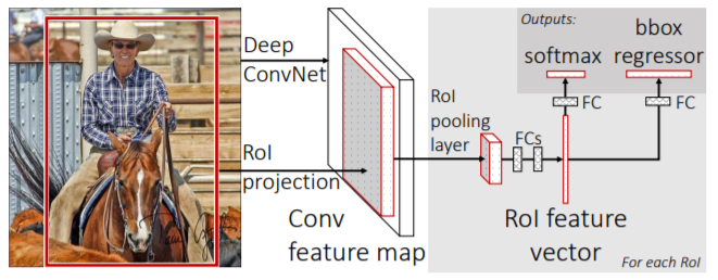
Image from Fast R-CNN
So, we can say that the main advantage of this solution is that it is possible to backpropagate through the whole network, and thus train it in an end-to-end manner. Both the training and testing phase are much faster than in R-CNN.
The inefficiency of backpropagation in R-CNN and SPPnet networks is due to the fact that each training sample (i.e. each RoI) comes from a different image, and since RoI may have a very large receptive field, the training inputs are very large (often the entire image).
In Fast RCNN training, stochastic gradient descent (SGD) minibatches are sampled hierarchically, first by sampling N images and then by sampling R/N RoIs from each image. Critically, RoIs from the same image share computation and memory in the forward and backward passes.
Moreover, if in R-CNN the softmax classifier, the SVMs and the regressors were trained in three different stages, in Fast R-CNN the softmax classifier and the bounding-box regressors are jointly optimized.
Notice also that in Fast R-CNN SVMs are no more used, substituted by the softmax classifier learnt during fine-tuning, since it was shown to perform a bit better.
One “problem”, however, is still present: it still depends on some external RoI extraction algorithm.
Faster R-CNN
Reference paper: Faster R-CNN: Towards Real-Time Object Detection with Region Proposal Networks
That is why Faster R-CNN was invented. Indeed, instead of the RoI extraction algorithm, a region proposal network (RPN) is used.
Our observation is that the convolutional (conv) feature maps used by region-based detectors, like Fast R-CNN, can also be used for generating region proposals. On top of these conv features, we construct RPNs by adding two additional conv layers: one that encodes each conv map position into a short (e.g., 256-d) feature vector and a second that, at each conv map position, outputs an objectness score and regressed bounds for k region proposals relative to various scales and aspect ratios at that location (k = 9 is a typical value).
Faster R-CNN: Towards Real-Time Object Detection with Region Proposal Networks
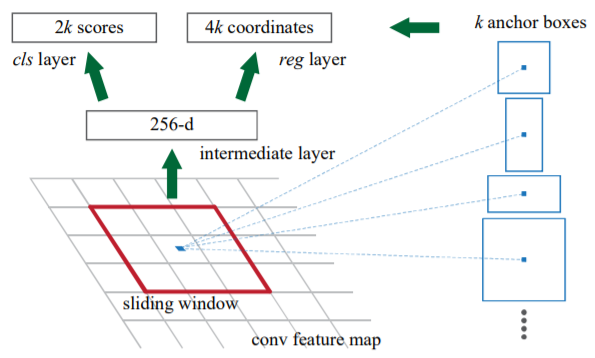
Image from Faster R-CNN: Towards Real-Time Object Detection with Region Proposal Networks
As we can see from the above image, a RPN takes as input an image of any size and outputs a set of object proposals, each with a objectness score, i.e. a measure of the membership to a set of object classes vs background. It is essentially a fully convolutional network, that maps each region to a lower-dimensional vector, which is then fed to two FC layers, one for classification and one for regression. Note that for each sliding window $k$ region proposals are simultaneously predicted, parameterized relative to $k$ different anchor boxes. Each anchor is centered at the sliding window and it is associated with a scale and aspect ratio. In the paper they used 3 scales and 3 aspect ratios, thus having 9 anchors for each sliding window. In general, if we consider a conv feature map of size $H \times W$, the total number of anchors is equal to $H \times W \times k$.
It is worth to show that now we have 4 losses:
- RPN classify object/non object
- RPN regression coordinates
- Final classification score
- Final BB coordinates
Apart from that, we can say that more or less the rest is a Fast R-CNN. At test time, indeed, we take the top $\sim 300$ anchors according to their object scores and we consider the refined BB locations of these 300 anchors. These are the RoI to be fed to a Fast R-CNN.
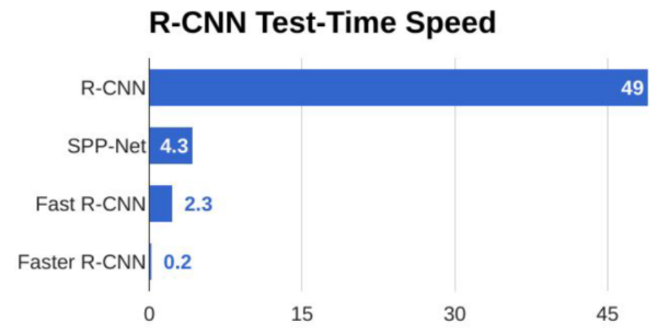
Comparison
YOLO/SSD
R-CNN methods are based on region proposals. However, there are also region-free methods, like:
- YOLO: You Only Look Once
- SSD: Single Shot Detectors
Reference paper: You Only Look Once: Unified, Real-Time Object Detection
Prior work on object detection repurposes classifiers to perform detection. Instead, we frame object detection as a regression problem to spatially separated bounding boxes and associated class probabilities. A single neural network predicts bounding boxes and class probabilities directly from full images in one evaluation. Since the whole detection pipeline is a single network, it can be optimized end-to-end directly on detection performance.
You Only Look Once: Unified, Real-Time Object Detection
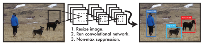
Image from You Only Look Once: Unified, Real-Time Object Detection
How does it work?
- Divide the input image into an $S \times S$ grid
If the center of an object falls into a grid cell, that grid cell is responsible for detecting that object.
- Each grid cell predicts $B$ bounding boxes and confidence score for those boxes. Confidence is defined as $Pr(Object) \cdot IOU_{pred}^{truth}$
- Each grid cell also predicts $C$ conditional class probabilities $Pr(class_i | Object)$
At test time the conditional class probabilities are multiplied by the individual box confidence predictions, so that the resulting scores encode both the probability of that class appearing in the box and how well the predicted box fits the object.
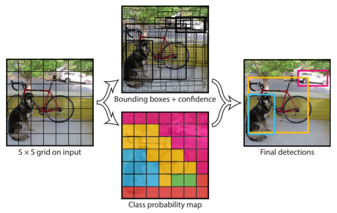
Image from You Only Look Once: Unified, Real-Time Object Detection
The network of YOLO is a “simple” CNN, inspired by the GoogLeNet model, with the convolutional layers pretrained on ImageNet.
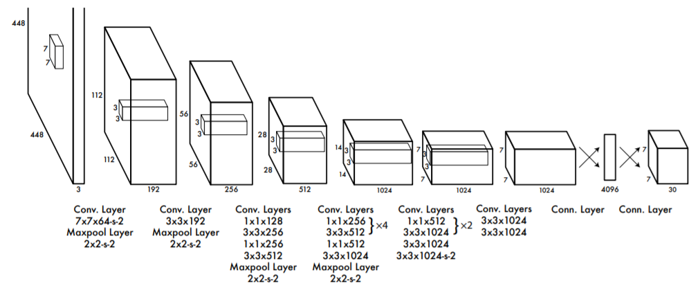
Image from You Only Look Once: Unified, Real-Time Object Detection
YOLO is incredibly faster than all the other methods we have seen. One limitation is that due to the spatial constraint imposed on the bounding box predictions (each grid cell can only have one class), the network struggles with small objects that appear in groups.
References
- B. Zhou, A. Khosla, A. Lapedriza, A. Oliva, A. Torralba - Learning Deep Features for Discriminative Localization
- R. Girshick, J. Donahue, T. Darrell, J. Malik - Rich feature hierarchies for accurate object detection and semantic segmentation
- Ross Girshick - Fast R-CNN
- S. Ren, K. He, R. Girshick, J. Sun - Faster R-CNN: Towards Real-Time Object Detection with Region Proposal Networks
- J. Redmon, S. Divvala, R. Girshick, A. Farhadi - You Only Look Once: Unified, Real-Time Object Detection
- Object Localization and Detection