In this post we will talk about the problem of overfitting, explaining what it is, what are its causes and how we can deal with it. More precisely, the following techniques will be explained: early stopping, weight decay and dropout.
Disclaimer: These notes are for the most part a collection of concepts taken from the slides of the ‘Artificial Neural Networks and Deep Learning’ course at Polytechnic of Milan, the book ‘Deep Learning’ (Goodfellow-et-al-2016) and from some other online resources. I am simply putting together all the information to study for the exam and I thought it would be a good idea to upload them here since they can be useful for someone who is interested in this topic.
Overfitting
Neural Networks are Universal Approximators
Universal Approximation Theorem:
“A single hidden layer feedforward neural network with S shaped activation functions can approximate any measurable function to any desired degree of accuracy on a compact set.” (Kurt Hornik, 1991)
If this is true, why do we always hear about neural networks with tens or even hundreds of hidden layers, with many different activation functions? Well, the theorem states that is possible, but…
- it doesn’t mean that we can find the necessary weights;
- an exponential number of hidden units may be required;
- it might be useless in practice if it does not generalize.
The last problem is called overfitting.
What is Overfitting?
In statistics, overfitting is “the production of an analysis that corresponds too closely or exactly to a particular set of data, and may therefore fail to fit additional data or predict future observations reliably” (Oxford Dictionaries).
The possibility of overfitting exists because the criterion used for selecting the model is not the same as the criterion used to judge the suitability of a model. For example, a model might be selected by maximizing its performance on some set of training data, and yet its suitability might be determined by its ability to perform well on unseen data; then overfitting occurs when a model begins to “memorize” training data rather than “learning” to generalize from a trend.
As an extreme example, if the number of parameters is the same as or greater than the number of observations, then a model can perfectly predict the training data simply by memorizing the data in its entirety. Such a model, though, will typically fail severely when making predictions.
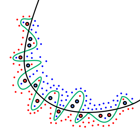
In the above image, the green line represents an overfitted model. Indeed, even if it is the one that best follows the training data, it is too dependent on that data, thus it will probably have an high error rate on unseen samples.
A more detailed view of this problem is described in the post Bias-Variance Tradeoff.
How can we measure generalization?
The training set error is not a valid measure of performance since it’s an optimistically biased estimate of the prediction error. The classifier, indeed, has been learned exactly on that data. Therefore, we need to test on an independent new test set.

How can we affect performance on the test set when we get to observe only the training set? If the training and the test set are collected arbitrarily, there is indeed little we can do. If we are allowed to make some assumptions about how the training and test set are collected, then we can make some progress. These assumptions are collectively known as the i.i.d. assumptions, and they imply that the examples in each dataset are independent from each other, and that the train set and the test set are identically distributed, i.e. drawn from the same probability distribution. This probabilistic framework and the i.i.d. assumptions allow us to mathematically study the relationship between training error and test error. [Deep Learning - pag. 111]
Note however that when we have to train a machine learning algorithm, the latter has many settings called hyperparameters (e.g. $\lambda$ in weight decay). In order to select the best value for each hyperparameter, we need a set of samples on which tune our model. That’s why, for the same reason that took us to split the dataset in training set and test set, it is good practice to split the dataset into one more set, called validation set.

Finally all the preparation is done. Summarizing:
- We train the model on the training set
- We evaluate the model on the validation set
- We tweak the model according to the results on validation set
- We select the model that performs best on validation set
- We test the model on the test set
Important: never train on test data!
Test sets and validation sets “wear out” with repeated use. That is, the more you use the same data to make decisions about hyperparameter settings or other model improvements, the less confidence you’ll have that these results actually generalize to new, unseen data. [Google ML crash course]
Cross-validation
When you have enough data, the method with the validation set described before is a good idea. However, when the dataset is too small you would like to not “waste” so many data that instead could be used for training. Cross-validation techniques solve exactly this problem:
Leave-Out-Out (LOO) cross-validation
A set of $n$ data points is repeatedly split into a training set containing all but one observation, and a validation set that contains only that observation. The test error is then estimated by averaging the $n$ resulting MSE’s.
$$ L_{LOO} = \frac{1}{N} \sum_{n=1}^{N} (t_n - y_{D \setminus {n}}(x_n))^2 $$
LOOCV generally gives the best result, but the price to pay is an high computational cost. If the dataset is small, it is the best approach (unless you are Google and you can use it even with a big dataset since the computational power is not a problem).
K-fold cross-validation
A set of $n$ observations is randomly split into $k$ non-overlapping groups. Each of these groups is used as a validation set, and the remainder as a training set. The test error is estimated by averaging the $k$ resulting MSE’s.
$$ L_{D_i} = \frac{k}{N} \sum_{(x_n,t_n) \in D} (t_n - y_{D \setminus {D_i}}(x_n))^2 $$
$$ L_{kfold} = \frac{1}{k} \sum_{i=1}^{k} L_{D_i} $$
K-fold cross-validation is much faster than LOO, but it is more (pessimistically) biased.
Early Stopping: Limiting Overfitting by Cross-validation
How can we know that our network is overfitting? Overfitting networks show a monotone training error trend (on average with SGD) as the number of gradient descent iterations $k$, but they lose generalization at some point…
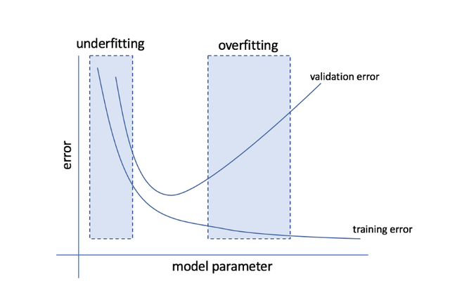
Image taken from https://towardsdatascience.com/cross-validation-70289113a072
Every time the error on the validation set improves, we store a copy of the model parameters. When the training algorithm terminates, we return these parameters, rather than the latest parameters. The algorithm terminates when no parameters have improved over the best recorded validation error for some pre-specified number of iterations. It is probably the most commonly used form of regularization in deep learning. Its popularity is due both to its effectiveness and its simplicity.
The only significant cost to choosing this hyperparameter automatically via early stopping is running the validation set evaluation periodically during training. Ideally, this is done in parallel to the training process on a separate machine, separate CPU, or separate GPU from the main training process.
Moreover, since early stopping requires a validation set, some training data are not fed to the model. To overcome this problem, we can perform an extra training procedure with all the data after the one with early stopping has finished. This extra training procedure can be done in two different ways:
- Initialize the model again and retrain with all the data for a number of steps equal to the one determined by the early stopping algorithm.
- Keep the parameters obtained from the early stopping algorithm and continue training with all the data. Note that this strategy has the advantage of not needing to retrain the model from scratch, but it is not guaranteed to terminate.
If you want to better understand How early stopping acts as a regularizer see the Deep Learning book at page 249. In few words, the idea is that by limiting the number of steps performed by the gradient descent in the loss function that we want to minimize, we are limiting the volume of parameter space reachable from an initial parameter. So we can say that somehow early stopping is similar to weight decay, but with the advantage that it can figure out for itself what is the right amount of regularization to apply, while weight decay needs to tune its $\lambda$ parameter (e.g. by cross-validation).
Weight Decay
I’ve already discussed this technique in another post –> Linear Regression
However, I will do it again here, adding some details.
Regularization is any modification we make to a learning algorithm that is intended to reduce its generalization error but not its training error. In case of weight decay, regularization consists of adding a penalty term to the loss function to discourage the coefficients from reaching large values.
So far we have maximized the data likelihood $w_{MLE} = argmax_w P(D|w)$. We can reduce the model “freedom” by introducing a prior distribution which influences the choice of the point estimate. This approach is called **Maximum A Posteriori (MAP)**:
$$ \theta_{MAP} = argmax_{\theta}\; p(\theta|x) = argmax_{\theta}\; log\; p(x|\theta) + log\; p(\theta) $$
where on the right hand side the first term is the likelihood and the second one the prior distribution.
Consider now a linear regression model with a Gaussian prior on the weights $P(w) \sim N(0,\sigma_w^2)$.
$$ \displaylines{\hat{w} = argmax_w P(w|D) = argmax_w P(D|w) P(w) \\ = argmax_w \prod_{n=1}^{N} \frac{1}{\sqrt{2\pi}\sigma} e^{-\frac{(t_n-g(x_n|w))^2}{2\sigma^2}} \prod_{q=1}^{Q} \frac{1}{\sqrt{2\pi}\sigma_w} e^{-\frac{(w_q)^2}{2\sigma_w^2}} \\ = argmin_w \sum_{n=1}^{N} \frac{(t_n-g(x_n|w))^2}{2\sigma^2} + \sum_{q=1}^{Q} \frac{(w_q)^2}{2\sigma_w^2} \\ = argmin_w \sum_{n=1}^{N} (t_n-g(x_n|w))^2 + \gamma \sum_{q=1}^{Q} (w_q)^2} $$
We thus have obtained a new loss function, where the second term represents the regularization. Minimizing this loss function results in a choice of weights that make a tradeoff between fitting the training data and being small. This gives us solutions that have a smaller slope, or put weight on fewer of the features.
Dropout
Dropout is one of the most simple but efficient techniques to regularize neural networks. The idea is pretty simple, but let’s make a premise: in machine learning there is one technique called bagging in which different models are trained through the use of bootstrapping. The main goal of this technique is to reduce the variance of the overall model, with the advantage that the training process is relatively easy to parallelize.
Ok, so one could think of using this approach also in neural networks. Here is the problem: with very large neural networks this becomes easily impractical. Dropout provides an inexpensive approximation to training and evaluating a bagged ensemble of exponentially many neural networks. By turning off randomly some neurons, we force to learn an independent feature preventing hidden units to rely on other units (co-adaptation). Specifically, to train with dropout, we use a minibatch-based learning algorithm that makes small steps, such as stochastic gradient descent. Each time we load an example into a minibatch, we randomly sample a different binary mask to apply to all of the input and hidden units in the network. The mask for each unit is sampled independently from all of the others. The probability of sampling a mask value of one (causing a unit to be included) is a hyperparameter fixed before training begins.
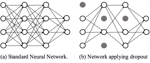
Image taken from Defensive Dropout for Hardening Deep Neural Networks under Adversarial Attacks
Note that there are two important differences between dropout and bagging:
-
In the case of bagging, the models are all independent. In the case of dropout the models share parameters, with each model inheriting a different subset of parameters from the parent neural network. This parameter sharing makes it possible to represent an exponential number of models with a tractable amount of memory.
-
In the case of bagging, each model is trained to convergence on its respective training set. In the case of dropout, typically most models are not explicitly trained at all—usually, the model is large enough that it would be infeasible to sample all possible subnetworks within the lifetime of the universe. Instead, a tiny fraction of the possible sub-networks are each trained for a single step, and the parameter sharing causes the remaining sub-networks to arrive at good settings of the parameters.
An interesting consequence of the fact that dropout trains not just a bagged ensemble of models, but an ensemble of models that share hidden units is that each hidden unit must be able to perform well regardless of which other hidden units are in the model. Hidden units must be prepared to be swapped and interchanged between models. Hinton et al. (2012c) were inspired by an idea from biology: sexual reproduction, which involves swapping genes between two different organisms, creates evolutionary pressure for genes to become not just good, but to become readily swapped between different organisms. Such genes and such features are very robust to changes in their environment because they are not able to incorrectly adapt to unusual features of any one organism or model. Dropout thus regularizes each hidden unit to be not merely a good feature but a feature that is good in many contexts.