The path followed in this post is: sequence-to-sequence models $\rightarrow$ neural turing machines $\rightarrow$ attentional interfaces $\rightarrow$ transformers. This post is dense of stuff, but I tried to keep it as simple as possible, without losing important details!

Disclaimer: These notes are for the most part a collection of concepts taken from the slides of the ‘Artificial Neural Networks and Deep Learning’ course at Polytechnic of Milan, the book ‘Deep Learning’ (Goodfellow-et-al-2016) and from some other online resources. I am simply putting together all the information to study for the exam and I thought it would be a good idea to upload them here since they can be useful for someone who is interested in this topic.

Sequence to Sequence Learning

As we can see from the below image, there are different sequential data problems:

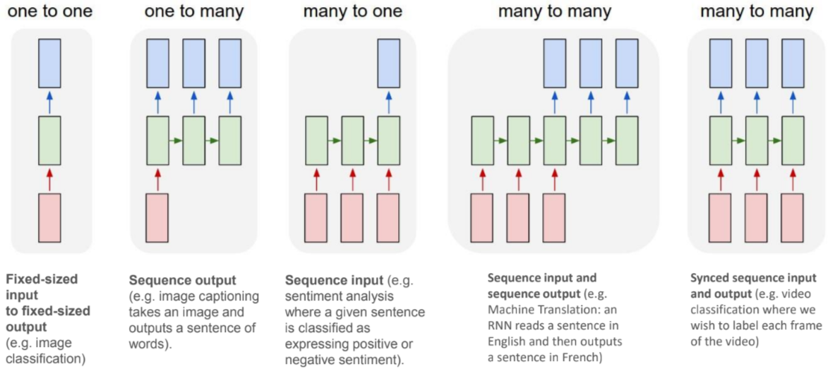
Credits Andrej Karpathy

In this post I want to discuss how a RNN can be trained to map an input sequence to an output sequence which is not necessarily of the same length. This model is at the core of many different tasks, like speech recognition, machine translation etc.

The first authors who proposed this new model (Cho et al. (2014) and Sutskever et al. (2014)) called it encoder-decoder or sequence-to-sequence architecture. The idea is pretty simple:

an encoder processes the input sequence and outputs an encoder vector represented by the final hidden state
a decoder takes as input the last hidden state of the encoder (the encoder vector) and produces the output sequence

During the training, the decoder does not feed the output of each time step to the next. The decoder input is the target sequence, here indicated in orange:

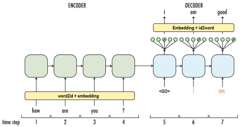
Credits Aj.Cheng

At inference time, instead, the decoder feeds the output of each time step as an input to the next one:

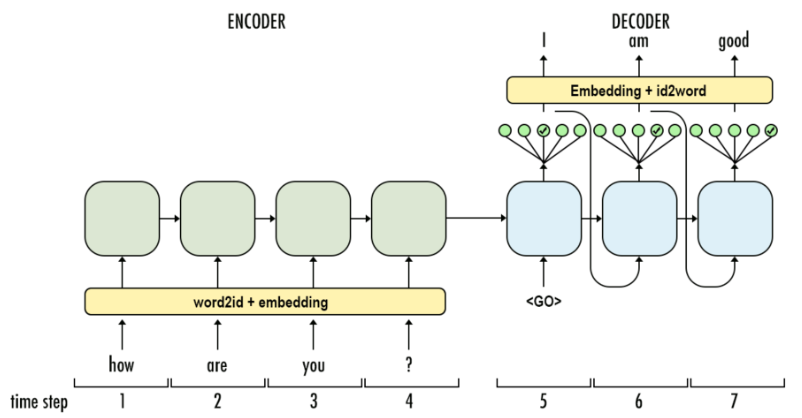
Credits Aj.Cheng

Dataset Batch Preparation

Sample batch_size pairs of (source_sequence, target_sequence)
Append <EOS> to the source_sequence
Prepend <SOS> to the target_sequence to obtain the target_input_sequence and append <EOS> to obtain target_output_sequence
Pad up to the max_input_length (max_target_length) withing the batch using the <PAD> token
Encode tokens based on vocabulary (or embedding)
Replace out of vocabulary (OOV) tokens with <UNK>. Compute the length of each input and target sequence in the batch

Extending Recurrent Neural Networks

Recurrent Neural Networks have been extended with memory to cope with very long sequences and also to deal with the encoding bottleneck present in the encoder-decoder architecture, which still imposes some limitations on how much knowledge/context we can embed in the encoder vector.

In this section I will use the awesome images of https://distill.pub/2016/augmented-rnns/, like the one below:

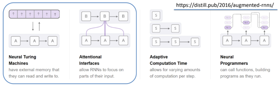
Credits https://distill.pub/2016/augmented-rnns/

As depicted, I will focus on the first two models.

Neural Turing Machines

Paper: Neural Turing Machines

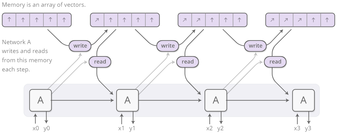
Credits https://distill.pub/2016/augmented-rnns/

The idea behind Neural Turing Machines is to enrich the capabilities of standard recurrent networks by adding an external memory, with which the model can interact using attentional mechanisms. The name comes from the analogy with the Turing’s operation of enriching finite-state-machines by adding an infinite memory tape.

The architecture of a NTM contains two basic components:

a controller, that interacts with the external environment taking inputs and giving outputs, and that also interacts with the memory through selective read and write operations.
a memory bank.

The main issue is: how can we make the whole differentiable? We want the read and write to be differentiable w.r.t. the location we read from or we write to, but this is not an easy task, since usually a single element in memory is addressed, like happens in Turing machine or in whatever digital computer. The authors of the paper came out with the following idea: let’s read and write in all the elements of the memory, but with a different degree in each cell. How? We can use attention.

Even if it can sound complicate, the attention mechanism is substantially a weighted average or if you prefer a distribution which indicates how we spread our “attention” over the memory locations. Let’s consider the read operation:

let $M_t$ be the memory matrix at time $t$, whose size is $N \times M$, where $N$ is the number of memory locations and $M$ is the vector size at each location
let $w_t$ be the weights over the $N$ locations at time $t$, such that $\sum_{i} w_t(i) = 1 \quad 0 \le w_t(i) \le 1; \forall i$

The result of the attention mechanism will be

$$ r_t \leftarrow \sum_{i} w_t(i) M_t(i) $$

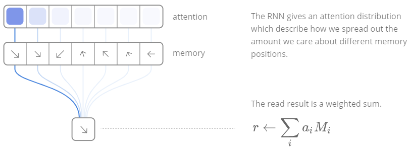
Credits https://distill.pub/2016/augmented-rnns/

The write operation, instead, takes inspiration from the input and forget gates of LSTMs:

1st step

$$ \tilde{M}_t(i) \leftarrow M_{t-1}(i) [\boldsymbol{1} - w_t(i)\boldsymbol{e_t}] $$

The formula is pretty intuitive: it is an update of the memory starting from its state at the previous time step. The interesting part is the second term of the multiplication: we have a row vector of all $1$s, from which we subtract the product between the weights and an erase vector $\boldsymbol{e_t}$, whose elements all lie in the range $(0,1)$. Thus, if either the weigthing or the erase is zero, the memory is left unchanged. On the other hand, if both the weigthing and the erase are one, the memory location is reset to zero.

2nd step

After the erase step, the add one is performed, in which an add vector $\boldsymbol{a_t}$ is added to the memory.

$$ M_t(i) \leftarrow \tilde{M}_t(i) + w_t(i) \boldsymbol{a_t} $$

Ok, but where do these weigthings come from? They are obtained by combining two addressing mechanisms:

content-based addressing

Content-based addressing focuses attention on locations based on the similarity between their current values and values emitted by the controller.

Neural Turing Machine
location-based addressing

However, not all problems are well-suited to content-based addressing. In certain tasks the content of a variable is arbitrary, but the variable still needs a recognisable name or address.

Neural Turing Machine

Go on https://distill.pub/2016/augmented-rnns/ to play with an amazing interactive figure in which you can observe the whole attention mechanism. I reported it here as a mere static image:

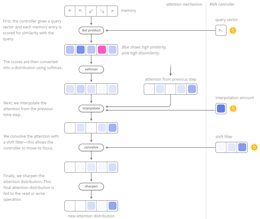
Credits https://distill.pub/2016/augmented-rnns/

Attentional Interfaces

Now that we have seen how Neural Turing Machines work, we won’t have any problem in applying the concept of attention to sequence-to-sequence models.

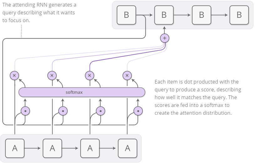
Credits https://distill.pub/2016/augmented-rnns/

If we consider for example the translation task, in the previous described sequence-to-sequence model we have to reduce the entire input sequence into a single vector and then expand it into the output translated sequence, losing meaningful information because of the bottleneck. Attention allows us to not lose this information by considering them all and then focusing on the most relevant ones for that specific time step.

Figure from Tensorflow Tutorial - NMT with attention

$$ \text{Attention weights:} \quad \quad \alpha_{ts} = \frac{exp(score(\boldsymbol{h_t}, \boldsymbol{\bar{h}_s}))}{\sum_{s'=1}^{S} exp(score(\boldsymbol{h_t}, \boldsymbol{\bar{h}_{s’}}))} $$

$$ \text{Context vector:} \quad \quad \boldsymbol{c_t} = \sum_{s} \alpha_{ts} \boldsymbol{\bar{h}_s} $$

$$ \text{Attention vector:} \quad \quad \boldsymbol{a_t} = f(\boldsymbol{c_t}, \boldsymbol{h_t}) = tanh(\boldsymbol{W_c}[\boldsymbol{c_t};\boldsymbol{h_t}]) $$

Transformers

In 2017 the Attention Is All You Need paper was published, introducing a new network architecture: the Transformer.

The inherently sequential nature precludes parallelization within training examples, which becomes critical at longer sequence lengths, as memory constraints limit batching across examples.

In this work we propose the Transformer, a model architecture eschewing recurrence and instead relying entirely on an attention mechanism to draw global dependencies between input and output. The Transformer allows for significantly more parallelization and can reach a new state of the art in translation quality after being trained for as little as twelve hours on eight P100 GPUs.

Important: in order to better understand transformers, I took inspiration from the awesome post http://jalammar.github.io/illustrated-transformer/

A Transformer model is made out of:

Scaled Dot-Product Attention
Multi-Head Attention
Position-wise Feed-Forward Networks
Embeddings and Softmax
Positional Encoding

Image from Attention Is All You Need

Let’s start with the first two components:

Scaled Dot-Product Attention and Multi-Head Attention

Image from Attention Is All You Need

The Scaled Dot-Product Attention is a particular attention that takes as input queries $Q$, keys $K$ and values $V$. These three matrices are obtained by multiplying our embeddings $X$ with some weights matrices $W^Q, W^K, W^V$ that we trained. The attention is then calculated as:

$$ Attention(Q,K,V) = softmax(\frac{QK^T}{\sqrt{d_k}})V $$

The reason for which they scale the dot products by $\sqrt{d_k}$ is

to counteract the fact that for large values of $d_k$ the dot products grow large in magnitude, pushing the softmax function into regions where it has extremely small gradients.

Now, this is the Scaled Dot-Product Attention. As we can see from the above image, taken from the paper, it is just a component of the Multi-Head Attention. Despite its name, Multi-Head Attention is exactly what we just said, but copied and pasted multiple times. We have indeed multiple sets of $Q, K, V$, one for each attention head (the Transformer has $8$ attention heads). This means that we will end up with $8$ matrices, so how can we feed them to the feed-forward layer? Attention function is performed in parallel and the resulting $d_v$-dimensional output values are concatenated, multiplied by a trained matrix $W^O$ and projected. Mathematically speaking:

$$ MultiHead(Q,K,V) = Concat(head_1,…,head_h) W^O $$

$$ head_i = Attention(QW_i^Q, KW_i^K, VW_i^V) $$

This multi-head attention is used in:

the encoder-decoder attention layers:

the queries come from the previous decoder layer, while the keys and values come from the output of the encoder, allowing every position in the decoder to attend over all positions in the input sequence.
the self-attention layers of the encoder:

each position in the encoder can attend to all positions in the previous layer of the encoder.
the self-attention layers of the decoder:

self-attention layers in the decoder allow each position in the decoder to attend to all positions in the decoder up to and including that position. This is obtained by setting to $-\infty$ all values in the input of the softmax that correspond to illegal connections.

Position-wise Feed-Forward Networks

The next component is the Position-wise Feed-Forward Networks, which is a standard fully connected feed-forward network contained in both the encoder and decoder. It consists of two linear transformations with a ReLU activation in between.

Positional Encoding

Positional encodings are added to the input embeddings in order to deal with the fact that, since the model does not contain any recurrence or convolution, there is the need to take into account the order of the sequence. There are different choices of positional encodings, in the paper they used sine and cosine functions of different frequencies.

Other observations

One layer which we did not discuss is the Add & Norm layer, in which through a residual connection the input embeddings are added to the result of the multi-head attention layer and then normalized.

The last two layers of the Transformer architecture are a linear layer and a softmax layer. Also in this case anything strange, the output of the decoder stack is a vector of floats, which goes through the linear layer, that flattens the vector into a very large logits vector (with size equal to our vocabulary). The final softmax layer transforms these values into probabilities.

Why Self attention

As written in the paper (section 4), there are different reasons to use self-attention, and I will try to summarize them here:

total computational complexity per layer
amount of computation that can be parallelized
path length between long-range dependencies in the network

Image from Attention Is All You Need

Seq2Seq models and the Attention mechanism

References

- Neural Turing Machines - Graves, Wayne, Danihelka - Google DeepMind
- Attention Is All You Need- NIPS 2017
- Olah & Carter, “Attention and Augmented Recurrent Neural Networks”, Distill, 2016
- Alammar, Jay (2018). The Illustrated Transformer [Blog post]
- Andrej Karpathy - RNN Effectiveness
- Aj.Cheng’s Medium post - Seq2Seq Models
- Tensorflow Tutorial - NMT with attention