In this post I will give you a brief introduction about Word Embedding, a technique used in NLP as an efficient representation of words.

Disclaimer: These notes are for the most part a collection of concepts taken from the slides of the ‘Artificial Neural Networks and Deep Learning’ course at Polytechnic of Milan and from some other online resources. I am simply putting together all the information to study for the exam and I thought it would be a good idea to upload them here since they can be useful for someone who is interested in this topic.

Word Embedding

Word embedding is the collective name for a set of language modeling and feature learning techniques in natural language processing (NLP) where words or phrases from the vocabulary are mapped to vectors of real numbers. Conceptually it involves a mathematical embedding from a space with many dimensions per word to a continuous vector space with a much lower dimension.

Wikipedia

The above description is pretty exaustive: we need an efficient way in which we can represent words so that they do not lose their meanings and relationships.

Before starting with word embedding, let’s see another approach: we can use a vector of size $V$ , where $V$ is the number of unique words in our dictionary, for each word, setting the position where that word is present to $1$ and all the others to $0$ .

	1	2	3	4
woman	1	0	0	0
cat	0	1	0	0
pizza	0	0	1	0
word	0	0	0	1

Now, you can guess how big this table would be if we consider a real dictionary. This method is called one-hot encoding and it is clear computationally unfeasible when $V$ is large. Moreover, notice that using this encoding we are losing the relationships between words: if for example we consider the words cat and dog, we would like them to be close in an hypothetical space of words, while instead in this representation they are orthogonal (cat $⊥$ dog), since their logical AND would result in a all zeros vector.

Word embeddings are much better, since they are short and dense. The fact that they are short and dense is useful not only from a computationally point of view, but also because containing fewer parameters they may generalize better, reducing the risk of overfitting. In addition to this, unlike one-hot-encoding, they do not lose the relationships between words, and they can even disclose hidden semantic relationships, like the fact that the relationship between cat and kitten is the same as the one between dog and puppy.

A Neural Probabilistic Language Model

Paper: A Neural Probabilistic Language Model

In 2003 Bengio at al. published this paper, in which they proposed a new model able to

fight the curse of dimensionality by learning a distributed representation for words which allows each training sentence to inform the model about an exponential number of semantically neighboring sentences.

reaching a clear improvement w.r.t. the previous state-of-the-art n-gram models.

In the model the training set is a sequence $w_{1}, \dots, w_{T}$ of words $w_{t} \in V$ , being $V$ a large vocabulary. The goal is to learn a good model $f (w_{t}, \dots, w_{t - n + 1}) = \hat{P} (w_{t} | w_{1}^{t - 1})$ , i.e. a model that outputs the most likely word given the previous ones. Such a function is decomposed in two parts:

a mapping $C$ from any element $i$ of $V$ to a real vector $C (i) \in R^{m}$
a function $g$ (it could be a feed-forward neural network) that maps an input sequence of feature vectors for words in context to a conditional probability distribution over words in $V$ for the next word $w_{t}$ :

$g (i, C (w_{t - 1}), \dots, C (w_{t - n + 1}))$

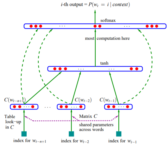
Image from A Neural Probabilistic Language Model

The reason for which I first described this model is that it is the base on which Mikolov et al. built what we know as Word2Vec.

Google’s Word2Vec

Paper: Efficient Estimation of Word Representations in Vector Space

In 2013 Mikolov at al. proposed two new model architectures for learning distributed representations of words that try to minimize computational complexity.

Continuous Bag-of-Words Model

CBOW is very similar to the Neural Network Language Model architecture briefly described before. The are three main differences:

the non-linear hidden layer is removed, and with it also most of the computational complexity
the projection layer is shared for all words (not just the projection matrix), thus all words get projected in the same position and their vectors are averaged
it also uses words from future

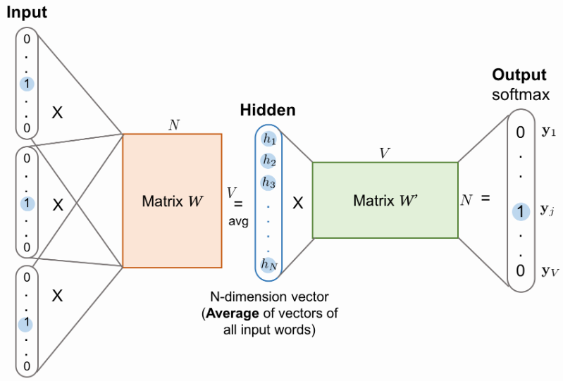
Credits https://lilianweng.github.io/lil-log/2017/10/15/learning-word-embedding.html

Continuous Skip-gram Model

The second architecture is similar to CBOW, but instead of predicting the current word based on the context, it tries to maximize classification of a word based on another word in the same sentence. More precisely, we use each current word as an input to a log-linear classifier with continuous projection layer, and predict words within a certain range before and after the current word.

Efficient Estimation of Word Representations in Vector Space

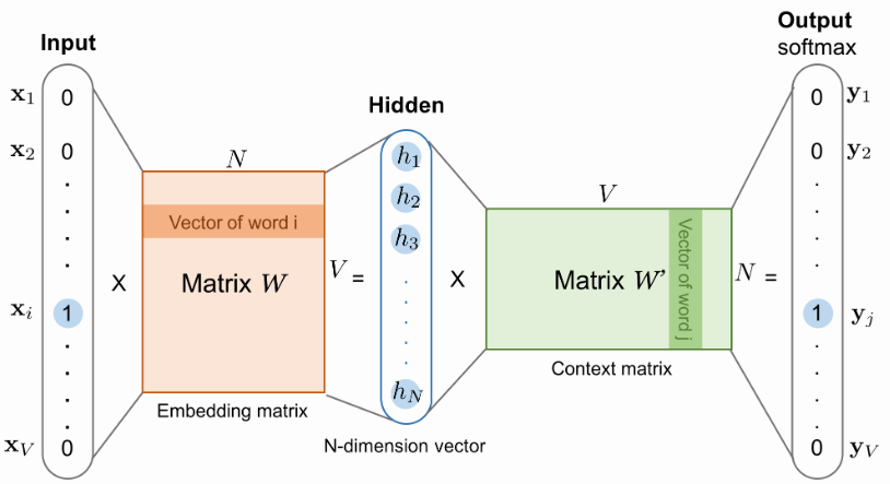
Credits https://lilianweng.github.io/lil-log/2017/10/15/learning-word-embedding.html

Essentially, the skip-gram model is trained to predict the probabilities of a word being a context word for the given target.

Note: the output context matrix $W^{'}$ encodes the meanings of words as context, different from the embedding matrix $W$ . Despite the name, $W^{'}$ is independent of $W$ , not a transpose or inverse or whatsoever.

Regularities in Word2Vec embedding space

Paper: Linguistic Regularities in Continuous Space Word Representations

It was shown that a simple method like the Vector Offset Method is very effective in solving analogy questions, like $a : b = c : d$ where $d$ is unknown. It works as follows: find the embedding vectors $x_{a}, x_{b}, x_{c}$ (all normalized to unit norm) and then compute $y = x_{b} - x_{a} + x_{c}$ . $y$ will be the continuous representation of the word we expect to be the best answer. Since no word might exist at that exact position, we search for the word whose embedding vector has the greatest cosine similarity to $y$ :

$w^{*} = a r g m a x_{w} \frac{x_{w} y}{| | x_{w} | | | | y | |}$

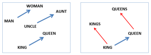
Image from Linguistic Regularities in Continuous Space Word Representations

Some interesting “semantic equations” that can be computed using embedding vectors are:

$\begin{matrix} w_{k i n g} - w_{m a n} + w_{w o m a n} ≅ w_{q u e e n} \\ w_{p a r i s} - w_{f r a n c e} + w_{i t a l y} ≅ w_{r o m e} \\ w_{e i n s t e i n} - w_{s c i e n t i s t} + w_{p a i n t e r} ≅ w_{p i c a s s o} \\ w_{h i s} - w_{h e} + w_{s h e} ≅ w_{h e r} \\ w_{c u} - w_{c o p p e r} + w_{g o l d} ≅ w_{a u} \end{matrix}$

GloVe

Paper: GloVe: Global Vectors for Word Representation

GloVe (Global Vectors) is another method for word embedding. It does explicitly what Word2Vec does implicitly, trying to extract meanings from co-occurence probabilities. Let’s see how it works:

$X$ is the matrix of word-word co-occurence counts, so that $X_{i j}$ representes the number of times the word $j$ occurs in the context of word $i$ .
$X_{i} = \sum_{k} X_{i k}$ is the number of times any word appears in the context of word $i$ .
$P_{i j} = P (j | i) = X i j / X_{i}$ is the probability that word $j$ appears in context of word $i$ .

Suppose for example that we have two words $i = i c e$ and $j = s t e a m$ . We can study the relationship between these two words by considering the ratio of their co-occurence probabilities with other words $k$ .

If we take a word related to $i c e$ but not related to $s t e a m$ , like $k = s o l i d$ , the ratio $\frac{P_{i k}}{P_{j k}}$ will be large. Viceversa, if $k$ is related to $s t e a m$ but not to $i c e$ , the ratio will be small. Finally, if $k$ is related to both or to neither, the ratio will be close to $1$ .

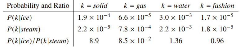
Table from Jeffrey Pennington, Richard Socher, Christopher D. Manning - GloVe: Global Vectors for Word Representation

The underlying idea is that the ratio is better than the mere probabilities at distinguish relevant words from irrelevant words. Thus, the most general model can be written as

$F (w_{i}, w_{j}, \tilde{w_{k}}) = \frac{P_{i k}}{P_{j k}}$

$F$ should be chosen so that it will encode the information coming from the ratio in the word vector space. One straightforward choice could be

$F (w_{i} - w_{j}, \tilde{w_{k}}) = \frac{P_{i k}}{P_{j k}}$

and then transforming its arguments in a scalar to match with the right-hand side term we obtain

$F ((w_{i} - w_{j})^{T} \tilde{w_{k}}) = \frac{P_{i k}}{P_{j k}}$

After this step, in the paper other transformations are applied, mainly in order to make the equation symmetric. If you are interested, please read the original paper for more details. For now, let’s consider the final equation, i.e.

$w_{i}^{T} {\tilde{w}}_{k} + b_{i} + {\tilde{b}}_{k} = \log (X_{i k})$

that actually becomes

$w_{i}^{T} {\tilde{w}}_{k} + b_{i} + {\tilde{b}}_{k} = \log (1 + X_{i k})$

to prevent the logarithm to diverge when its argument is zero.

This model, however, has the problem of weighting all co-occurences equally, no matter if they happen rarely or never. To address this problem a specific loss function is used:

$J = \sum_{i, j = 1}^{V} f (X_{i j}) (w_{i}^{T} {\tilde{w}}_{j} + b_{i} + {\tilde{b}}_{j} - l o g X_{i j})^{2}$

where $f (X_{i j})$ is a weighting function with some interesting properties in order to deal with rare and frequent co-occurences (again, read the paper for more details).

Word Embedding#

A Neural Probabilistic Language Model#

Google’s Word2Vec#

Continuous Bag-of-Words Model#

Continuous Skip-gram Model#

Regularities in Word2Vec embedding space#

GloVe#

References#